Simulation Details¶

Including the required Python libraries¶

Python libraries are included in a file by placing

import PythonLibrary as pl

at the beginning of the file. Here, PythonLibrary is the name of the Python library to be included, and pl is the namespace where the contents of this module are placed. As an example, if we wanted to include MPSPyLib and call the function Ops.BuildSpinOperators() from this library, we would use the code

import MPSPyLib as mps
Operators = mps.BuildSpinOperators()

Note the use of the namespace identifier mps to specify that Ops.BuildSpinOperators() comes from MPSPyLib. In addition to MPSPyLib, which is always required for MPS simulations, we will also frequently include NumPy, as it provides the matrix functionality used internally for the code. We will use the namespace identifier np for NumPy.

Specifying the parameters of a simulation¶

A simulation is specified in MPSPyLib as a Python dictionary of simulation data. A Python dictionary, also called a hash table, is an unordered collection of key:value pairs. For example, we could construct a dictionary which has a single key 'name' which maps to the string 'fred' as

mydict = {'name' : 'fred'}

A dictionary is specified by curly braces, $\{ \ldots \}$ , with key:value pairs separated by a colon, :, which assigns each key to a value. In python dictionaries, the keys can be any type of immutable data (i.e. strings, tuples, or numbers). Each key must be unique to the dictionary. The values assigned to each key is not necessarily unique, and can be any data type. The value corresponding to a key is accessed by calling that element of the dictionary using square brackets, $\left[ \ldots \right]$ , referring to the dictionary name mydict and the key 'name' with the command mydict['name'].

We will refer to the Python dictionary specifying a simulation in MPSPyLib as parameters. Every simulation must have the non-optional keys listed in the table in tools.WriteFiles(). Furthermore optional parameters are available if the default values are not suitable for the goal of the simulation. The particular choice of these parameters defines which algorithms are to be used and their convergence properties. In addition, parameters should also contain the values of the Hamiltonian parameters used to define the Hamiltonian, see Sec. Defining the Hamiltonian and other many-body operators. The simulation specification parameters is converted into simulation data which is readable by the Fortran backend using the function

MainFiles = mps.WriteFiles(parameters, Operators, H)

where Operators specifies the operators defining the on-site Hilbert space, see Sec. Defining local operators, and H specifies the Hamiltonian, see Sec. Defining the Hamiltonian and other many-body operators. The specification of simulations parameters can also be a list of dictionaries, which allows for easy batching and parallelization of simulations. A full set of examples are included in the Examples subdirectory of OSMPS.

Defining local operators¶

Overview of operators in MPSPyLib¶

The way that ordinary, meaning non-symmetry-adapted, operators are stored in MPSPyLib are as dictionaries, which are unordered collections of key:value pairs (Symmetry-adapted operators are discussed in Sec. Abelian symmetries). This means that the set of operators is stored as a dictionary, call it Operators, and

Operators['tag']

returns the matrix representation of the operator 'tag' as a NumPy array. The default operators built by the convenience functions are listed in a table inside of the function description. 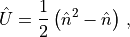The options are spin operators from Ops.BuildSpinOperators(), bosonic operators defined in Ops.BuildBoseOperators(), fermionic operators created by the function Ops.BuildFermiOperators(), or operators for a Bose-Fermi system Ops.BuildFermiBoseOperators() building all operators present in the bosonic and fermionic set. The total number operator $\hat{n}$ with the key 'ntotal' is built in addition for the latter one. For more information on the optional arguments of these functions, one can use the help functionality of Python as alternative to this documentation, e.g.

help(mps.BuildBoseOperators)

within the Python interpreter.

New operators can be defined by arithmetic on existing operators, and the new operator is designated by a user-defined key. As an example, consider that one wants to construct the bosonic on-site interaction operator

$\hat{U} &= \frac{1}{2} \left( \hat{n}^2 - \hat{n} \right) \, ,$

and call it 'Interaction'. This may be achieved as

import MPSPyLib as mps
import numpy as np

Operators = mps.BuildBoseOperators(Nmax=2)
Operators['Interaction'] = 0.5 * (np.dot(Operators['nbtotal'], Operators['nbtotal']) - Operators['nbtotal'])

Here, np.dot is matrix-matrix multiplication from the NumPy libraries.

Operators with internal degrees of freedom¶

MPSPyLib contains two different methods for generating operators for particles with internal degrees of freedom. The first is to include a value for the spin of the particle in Ops.BuildBoseOperators() or Ops.BuildFermiOperators(). In that case each operator from the set of operators, with the exception of the total number and Fermi phase operators, obtains a spin projection index e.g. tag_m, where m runs from 0 to $2s$ , with $s$ the spin. In addition, the number operators in each component n*_m and the spin operators '*sz, '*splus, and '*sminus are built, where *=b for bosons and *=f for fermions.

The second means of producing particles with internal degrees of freedom in MPSPyLib is through specifying a nonzero value for the nFlavors optional argument of Ops.BuildBoseOperators() or Ops.BuildFermiOperators(). In this case each operator from the set of operators, with the exception of the total number operator, obtains a flavor projection index e.g. tag_m, where m runs from 0 to nFlavors-1, and the number operators in each component n*\_m are built, where *=b for bosons and *=f for fermions. If both spin and nFlavors are nonzero, then the operators are indexed as 'tag\_flavor\_m', where flavor runs from 0 to nFlavors-1 and m runs from 0 to $2s$ , with $s$ the spin. In Ops.BuildFermiBoseOperators() different flavors and spins can be specified for the bosonic and fermionic species. For more information on this syntax consult the docstring for Ops.BuildFermiBoseOperators().

Finally, we note that the matrix representations of the operators may be viewed by using the print functionality of python. That is, if we wanted to see the bosonic destruction operator b, we could call

import MPSPyLib as mps
import numpy as np

Operators = mps.BuildBoseOperators(Nmax=2)
print(Operators['b'])

Likewise, we can print all the operators as

for i in Operators:
    print(Operators[i])

Defining the Hamiltonian and other many-body operators¶

Matrix Product Operators¶

The matrix product operators organize the class mpo.MPO. The natural operator structure for MPS algorithms is a matrix product operator (MPO). The exact diagonalization modules uses the same class to construct Hamiltonians, effective Hamiltonians, and operators in Liouville space. Operators can be constructed as MPOs using a set of rules which specify how operators acting on local Hilbert spaces are combined to create an operator acting on the entire many-body system. Using a canonical form for MPOs, several operators constructed from these rules can be put together as a single MPO [WC12]. OSMPS uses this essential idea of creating operators from a set of predetermined rules to construct the Hamiltonian and other operators appearing in an MPS simulation.

An operator acting on the many-body state, i.e. the MPO, is an object of the mpo.MPO class in MPSPyLib. For an instantiation of the MPO class, named H in the following, is obtained as

H = mps.MPO(Operators)

Once we have an MPO object, we add terms to it using the Ops.AddMPOTerm() method. In particular, the rules are defined in the module mpoterm.

MPO Terms to build rule sets¶

The following MPO terms are available at present

site rule (mpoterm.SiteTerm). Example:

H.AddMPOTerm('site', 'sz', hparam='h_z', weight=1.0)
generates $\hat{H}=h_z\sum_{i=1}^{L}\hat{S}^z_i$ , where $\hat{S}^z =$ Operators['sz']} and Operators was already passed when creating the instance of the MPO. The second argument contains the relevant keys of the operators to be used. Because only the names of the operators are used, this routine handles ordinary and symmetry-adapted operators on the same footing.

bond rule (mpoterm.BondTerm). Example:

H.AddMPOTerm('bond', ['splus','sminus'], hparam='J_xy', weight=0.5)
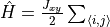
generates $\hat{H} = \frac{J_{xy}}{2} \sum_{\langle i,j \rangle}$ $\left(\hat{S}^{+}_{i} \hat{S}^{-}_{j} + \mathrm{h.c.} \right)$ , where $\langle i,j\rangle$ denotes all nearest neighbor pairs $i$ and $j$ ,
H.AddMPOTerm('bond', ['sz', 'sz'], hparam='J_z', weight=1.0)
generates $\hat{H}=J_{z}\sum_{\langle i,j\rangle}\hat{S}^z_i\hat{S}^z_j$ , and
H.AddMPOTerm('bond', ['fdagger', 'f'], hparam='t', weight=-1.0, Phase=True)
generates $\hat{H} = -t \sum_{\langle i,j \rangle}$ $\left(\hat{f}_i^{\dagger} \hat{f}_j + \mathrm{h.c.} \right)$ , where $\hat{f}$ is a fermionic destruction operator. That is, terms with Fermi phases are cared for with the optional Phase argument and Hermiticity is automatically enforced by this routine. The Fermi phase is added through a Jordan-Wigner string of the operators in Operator with key FermiPhase. The functions Ops.BuildFermiOperators() and Ops.BuildFermiBoseOperators() discussed in Sec. Defining local operators both create the Fermi phase operator appropriate for this use automatically. Notice that the order of the operators matters due to the Jordan-Wigner transformation. Adding ['f', 'fdagger'] does not result in the same fermionic Hamiltonian. A warning will be printed for obvious cases.

exponential rule set (mpoterm.ExpTerm). Example

H.AddMPOTerm('exponential', ['sz', 'sz'], hparam='J_z', decayparam=a, weight=1.0)
generates $\hat{H} =J_z \sum_{i<j} a^{j-i+1} \hat{S}^z_i \hat{S}^z_j$ . This rule also enforces Hermiticity and cares for Fermi phases as in the bond rule case.

FiniteFunction rule (mpoterm.FiniteFunc). Example:

f = []
for ii in range(6):
    f.append(1.0 / (ii + 1.0)**3)
H.AddMPOTerm('FiniteFunction', ['sz', 'sz'], f=f, hparam='J_z', weight=-1.0)
generates $\hat{H} = -J_z \sum_{1 \le i,j \le 6}$ $\frac{1}{\left|j-i \right|^3} \hat{S}^z_i \hat{S}^z_j$ , where the summation is over all $i$ and $j$ pairs separated by at least $1$ and at most $6$ lattice spacings. The range of the potential is given by the number of elements in the list f. This rule enforces Hermiticity and cares for Fermi phases as in the bond rule case.

InfiniteFunction rule set (mpoterm.InfiniteFunc). We point out that this term is always fitted with a set of mpoterm.ExpTerm for MPS simulations. Examples:

invrcube = lambda x: 1.0/(x*x*x)
H.AddMPOTerm('InfiniteFunction', ['sz', 'sz'], hparam='J_z', weight=1.0,
             func=invrcube, L=1000, tol=1e-9)
generates $\hat{H}=\sum_{i<j}\frac{1}{\left|j-i\right|^3}\hat{S}^z_i\hat{S}^z_j$ , where the functional form is valid to a distance L with a residual of at most tol. Similarly,
H.AddMPOTerm('InfiniteFunction', ['sz', 'sz'], hparam='J_z', weight=1.0, 
             x=x, y=f, tol=1e-9)
generates $\hat{H}=\sum_{i<j}f\left(j-i\right)\hat{S}^z_i\hat{S}^z_j$ , where the functional form $f\left(x\right)$ is determined by the array of values f and the array of evaluation points x. The distance of validity L is determined from the array x. This rule applies only to monotonically decreasing functions func or f, and so outside the range of validity L the corrections are also monotonically decreasing. This rule enforces Hermiticity and cares for Fermi phases as in the bond rule case.

product rule (mpoterm.ProductTerm). Example:

H.AddMPOTerm('product', 'sz', hparam='h_p', weight=-1.0)
generates $\hat{H}=-h_p\prod_{i=1}^{L} \hat{S}^z_i$ . The operator used in the product must be Hermitian.

MBString rule set(mpoterm.MBStringTerm). See function description for usage.
mpoterm.TTerm. See function description for usage.
mpoterm.SiteLindXX. See function description for usage.
mpoterm.LindExp. See function description for usage.
mpoterm.LindInfFunc. See function description for usage.
mpoterm.MBSLind. See function description for usage. (Can act as nearest neighbor Lindblad term.)

In all of the above expressions, H is an object of the MPO class. The strings passed to the argument hparams represent tags for variable Hamiltonian parameters, which allow for easy batching and parallelization (Sec. Running a parallel static simulation), and also facilitate dynamical processes The argument hparams is optional, and defaults to the constant value 1. The optional argument weight specifies a constant factor that scales the operator and defaults to the value 1, too.

Developer’s Guide for Rule Sets

Module contains a class for each possible term in the MPO rule sets. Each term is derived from a base class.If you plan to add additional MPO terms to OSMPS, you have to modify the following files. In the case of a new Lindblad operator, these are

mpoterm.py: add class for the new term
mpo.py: add new term to the MPO structure and enable writing.
MPOOps_types_templates.f90: define derived type and add to MPORuleSet
MPOOps_include.f90: add read/destroy methods for RuleSets
MPOOps_include.f90: effective Hamiltonian for 2 sites
MPOOps_include.f90: Liouville operator for 2 sites
MPOOps_include.f90: effective Hamiltonian represented as MPO.
MPOOps_include.f90: Liouville operator represented as MPO.
TimeevolutionOps_include.f90: Add overlaps to QT functionality.

Example

As an example, a template MPO for the Hamiltonian of the hard-core boson model with $1/r^3$ interactions,

$\hat{H} &= -t \sum_{\langle i,j \rangle} \left(\hat{b}_i^{\dagger} \hat{b}_j + \mathrm{h.c.} \right) + U \sum_{i<j} \frac{\hat{n}_i \hat{n}_j}{\left|j-i \right|^3} - \mu \sum_{i} \hat{n}_i \, ,$

is provided by

import MPSPyLib as mps

# Build operators
Operators = mps.BuildBoseOperators(1)
# Define Hamiltonian MPO
H = mps.MPO(Operators)
H.AddMPOTerm('site', 'nbtotal', hparam='mu', weight=-1.0)
H.AddMPOTerm('bond', ['bdagger', 'b'], hparam='t', weight=-1.0)
invrcube = lambda x: 1.0/(x*x*x)
H.AddMPOTerm('InfiniteFunction', ['nbtotal', 'nbtotal'], hparam='U',
             weight=1.0, func=invrcube, L=1000, tol=1e-9)

We stress that no assumptions are made about the hparam parameters 't', 'mu', or 'U' when the MPO is built. The hparams are simply tags parameterizing the operators which appear in the Hamiltonian. The actual numerical values of $t$ , $U$ , and $\mu$ are specified as part of the dictionary parameters discussed in Sec. Specifying the parameters of a simulation. These parameters can also be position-dependent, as demonstrated in the example files in OpenMPS Examples.

One can print operators using the mpo.MPO.printMPO() method. As an example, the interacting spinless fermion model

$\hat{H} &= - t \sum_{\langle i,j \rangle} \left(\hat{f}_i^{\dagger} \hat{f}_j + \mathrm{h.c.} \right) + U\sum_{\langle i,j \rangle }{\hat{n}_i \hat{n}_j} \, ,$

is specified and printed as

import MPSPyLib as mps

# Build operators
Operators = mps.BuildFermiOperators()
# Define Hamiltonian MPO
H = mps.MPO(Operators)
H.AddMPOTerm('bond', ['fdagger', 'f'], hparam='t', weight=-1.0, Phase=True)
H.AddMPOTerm('bond', ['nftotal', 'nftotal'], hparam='U', weight=1.0)
H.printMPO()

The result of this code is

-1.0 * t * sum_i fdaggerP_i f_{i+1} + 1.0 * t * sum_i fP_i fdaggerP_{i+1} + 1.0 * U * sum_i nftotal_i nftotal_{i+1}

Note the use of the phased operators fdaggerP and fP according to Phase=True.

As the 'InfiniteFunction' rule constructs MPOs by fitting the decaying function to a series of weighted exponentials, the result of printMPO will contain the data for the exponentials and not information about the infinite function proper.

Finally, as complex MPOs with InfiniteFunction interactions can be expensive to generate, one can save the data in an MPO object instance using the mpo.WriteMPO() function, and then read it in later using the mpo.ReadMPO() function. The syntax for these is

mps.WriteMPO(H,filename)
H = mps.ReadMPO(filename)

where H is an object of the mpo.MPO class and filename is the name of the file where the MPO is written to/read from.

Defining and reading observables: `obsterms.Observables`¶

Defining Observables¶

Module obsterms defines the observables on quantum systems. Each observable contains the corresponding methods to write the fortran files and to read the results from the fortran outputs. The following observables are defined

Observables on any quantum sytem in OSMPS are specified by instantiating an object of the obsterms.Observables class, for example

myObservables = Observables(Operators)

One then adds observables using the obsterms.Observables.AddObservable() method. Each observable is itself a python class and has the corresponding read/write methods Examples of the use of obsterms.Observables.AddObservable() are:

site observables (obsterms.SiteObservable). Example :

myObservables.AddObservable('site', 'nbtotal', name='n')
will measure $\langle \hat{n} \rangle$ at each site and return the result as a length- $L$ vector with the tag 'n'. Recall that $L$ is either the system size in the case of a finite MPS or the unit cell length in the case of iMPS as specified in the table in the description of WriteFiles()

Site entropy measurement (obsterms.SiteEntropyObservable).
Bond entropy measurement (obsterms.BondEntropyObservable).
corr observables (obsterms.CorrObservable and obsterms.FCorrObservable). Example:

myObservables.AddObservable('corr', ['nbtotal', 'nbtotal'], name='nn')
will measure $\langle \hat{n}_i \hat{n}_j \rangle$ at each independent pair of sites $i \le j$ and return the result with the tag 'nn'. For finite-size MPS simulations the result is returned as an $L imes L$ matrix, and for infinite-size MPS simulations the result is returned as a length- $L$ vector, where $L$ is specified by the SpecifyCorrelationRange method, see Sec. Infinite-size ground state search: iMPS. For observables involving odd numbers of fermionic operators on a given site, there is an optional Phase argument such as existed for the mpo.MPO.AddMPOTerm() method. An example is
myObservables.AddObservable('corr', ['fdagger', 'f'], name='spdm', 
                            Phase=True)
which measures the fermionic correlation function $\langle \hat{f}_i^{\dagger}\hat{f}_j \rangle$ .

string observables (obsterms.StringCorrObservable). Example (from Infiniteheisenbergspinone.py):

myObservables.AddObservable('string', ['sz', 'sz', 'phaseString'], 
                            name='StringOP')
will measure $\langle \hat{S}^z_i\prod_{k=i+1}^{j-1}\left(-1 \right)^{i\pi \hat{S}^z_k}\hat{S}^z_j \rangle$ at each independent pair of sites $i\le j$ and return the result with the tag 'StringOP'. Note that phaseString has been defined to be $\left(-1 \right)^{i\pi \hat{S}^z_k}$ only in this particular case.

MPO observables (obsterms.MPOObservable). Example:

DefectDensity = mps.MPO(Operators)
DefectDensity.AddMPOTerm('bond', ['sz', 'sz'])
myStaticObservables.AddObservable('MPO', DefectDensity, 'Defect Density')
will measure $\sum_{\langle i,j \rangle}\hat{S}^z_i\hat{S}^z_j$ and return the result with the tag 'Defect Density'. In this way, essentially arbitrary many-body operators may be measured.

Reduced density matrix, limited to one (obsterms.RhoiObservable) or two (obsterms.RhoijObservable) sites at present, can be measured as well. They can be added once as single item or list. An empty list indicates to report the singular values at all bipartitions. If passed as list, entries have to sorted ascending.

myObservables.AddObservables('DensityMatrix_i', [])
myObservables.AddObservables('DensityMatrix_ij', [])

It is possible to measure the mutual information matrix without writing all the information about the reduced density matrices to the result files (obsterms.MutualInformationObservable).
```
myObservables.AddObservables('MI', True)
```
The Schmidt values (obsterms.LambdaObservable) at the bipartitions are another measurement, which gives a more detailed picture than the bond entropy. They can be added once as single item or list. An empty list indicates to report the singular values at all bipartitions.

myObservables.AddObservables('Lambda', [])

Distance to a pure state (obsterms.DistancePsiObs)
Save state independent from checkpoints etc. (MPS only, obsterms.StateObservable)
Gate observables (ED only, obsterms.GateObservable).
Distance to a density matrix (ED only, obsterms.DistanceRhoObs).

Observables for the different algorithms in OSMPS are specified as part of the parameters dictionary, see Table in tools.WriteFiles().

Developer’s Guide for new observables

Implement new class in this module, i.e. obsterms. We need the minimal class functions __init__, add, write, and read.
Add new observable to the data set and mpslist in :py:class:Observables.
Modify ObsOps_types_templates.f90 by adding a new observable to OBS_TYPE and possibly defining a new derived type for this observable.
Define read, write, and destroy methods as far as applicable.
Carry out measurements in all observe subroutines.

Reading Observables¶

The observables which correspond to static algorithms such as MPS and eMPS, see Sec. Algorithms of the OpenMPS, are read using the obsterms.ReadStaticObservables() function taking the parameters dictionary as argument. Here, the observables for MPS are specified by the key 'MPSObservables' in 'parameters' and, similarly, the key 'eMPSObservables' in 'parameters' specifies the observables for eMPS, see Table in tools.WriteFiles(). The output from obsterms.ReadStaticObservables() is a list of dictionaries. The number of elements in the list is equal to the number of individual simulations. An element of this list contains all of the relevant simulation metadata from parameters as well as the observables specified in myObservables with the tags given by the obsterms.Observables.AddObservable() method. That is, Output['n'] outputs the observable 'n' as tagged by obsterms.Observables.AddObservable() for the dictionary Output which is an element of Outputs. The tags of the various default information returned from obsterms.ReadStaticObservables() can be found in the function documentation.

In addition to the observables which are specified using the obsterms.Observables.AddObservable() method, the von Neumann entropy of entanglement of a given site $i$ with the rest of the system,

$S_{\mathrm{site},i}&\equiv -\mathrm{Tr}\left[\hat{\rho}_i\log\hat{\rho}_i\right]\, ,\;\;\; \hat{\rho}_i\equiv \mathrm{Tr}_{j\ne i}|\psi\rangle\langle \psi|$

is measured whenever not deactivated. The result is stored as an $L$ -length vector with the tag 'SiteEntropy'. Additionally, the von Neumann entropy of entanglement of bipartition $i$

$S_{\mathrm{bond},i}&\equiv -\mathrm{Tr}\left[\hat{\rho}_i\log\hat{\rho}_i\right]\, ,\;\;\; \hat{\rho}_i\equiv \mathrm{Tr}_{j\ge i}|\psi\rangle\langle \psi|$

is measured whenever not deactivated. For finite-size MPS simulations, the result is stored as an $\left(L+1\right)$ -length vector with the tag 'BondEntropy'. For infinite-size MPS simulations, 'BondEntropy' is always measured, and is a scalar indicating the entropy of entanglement of the bipartition between any two adjacent unit cells.

For finite-size systems, the total energy 'energy' and the variance 'variance' $\equiv\langle \hat{H}^2-E^2\rangle$ are always measured. The quantity 'converged' returns a value of 'T' or 'F' depending on whether the variance met the desired user-defined tolerance or not, respectively. For infinite-sized systems, the energy is replaced by 'energy_density', and the 'convergence' is determined from the orthogonality fidelity as discussed in Sec. Infinite-size ground state search: iMPS. Finally, in all cases, the maximum bond dimension of the MPS is returned as 'bond_dimension'.

To extract observables from tMPS simulations, the function obsterms.ReadDynamicObservables() taking the paramaeters dictionary as argument is used. The observables for tMPS are specified by the key 'DynamicsObservables' in 'parameters'. The default observables returned from obsterms.ReadDynamicObservables() are given in its function description. The number of elements of Outputs corresponds to the number of elements of parameters, but each element of Outputs is itself a list whose length is the number of time steps. These elements are distinguished by the key 'time'. Time is measured in units of $\hbar/E_{\mathrm{unit}}$ , where $E_{\mathrm{unit}}$ is the unit of energy set by the magnitudes of the Hamiltonian parameters.

Specification of dynamics¶

A dynamical process simulated with tMPS, details on the algorithms can be found starting at Sec. Krylov-based time evolution : tMPS, is specified as an object of the Dynamics.QuenchList class. An object of this class is obtained as

Quenches = mps.QuenchList(H)

where H is an MPO.MPO object specifying the MPO of the Hamiltonian used to time-evolve the state. Dynamical processes, which we will call quenches, are added using the Dynamics.QuenchList.AddQuench() method with the syntax

Quenches.AddQuench(Hparams, time, deltat, funcs, ConvergenceParameters=None, stepsforoutput=1)

Here Hparams is a list of the tags of the Hamiltonian parameters in H which are to be modified during the quench, time is the total time of this quench, deltat is the desired numerical time step, funcs is a list of functions specifying how the Hamiltonian parameters given in Hparams change in time. ConvergenceParameters is used to specify the time evolution algorithm used and its convergence parameters for this quench. The available options are the convergence.KrylovConvParam, convergence.TEBDConvParam, convergence.TDVPConvParam. and convergence.LRKConvParam. Finally, stepsforoutput denotes the number time steps between measurements of the state. The functions in funcs should take a single argument which is the time. At present, dynamics always begins from the ground state, and the Hamiltonian used for time evolution must have the same form as the Hamiltonian used for dynamics. That is, the two Hamiltonians must have the same Hamiltonian parameters and these parameters must be of the same numerical type, e.g. if a parameter is site-dependent for statics it must also be site-dependent for dynamics and vice versa.

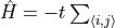
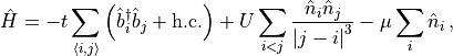
It is useful here to consider a specific example. We consider quenching the parameter $U$ in the Bose-Hubbard model

$\hat{H}&=-t\sum_{\langle i,j\rangle}\left[\hat{b}_i^{\dagger}\hat{b}_j+\mathrm{h.c.}\right]+U\sum_{i}\frac{\hat{n}_i\left(\hat{n}_i-1\right)}{2}$

linearly from 10 to 1, and then linearly back to 10 over a time $\tau$ . Using the Hamiltonian specification

Operators = mps.BuildBoseOperators(5)
Operators['interaction'] = 0.5 * (np.dot(Operators['nbtotal'], Operators['nbtotal']) - Operators['nbtotal'])
H = mps.MPO(Operators)
H.AddMPOTerm('bond', ['bdagger', 'b'], hparam='t', weight=-1.0)
H.AddMPOTerm('site', 'interaction', hparam='U', weight=1.0)

this quench process is generated as

# Quench function ramping down
def Ufuncdown(t, tau=tau):
     return 10.0 + 2.0 * (1.0 - 10.0) * t / tau

# Quench function ramping back up
def Ufuncup(t, tau=tau):
    return 1.0 + 2.0 * (10.0 - 1.0) * (t - 0.5 * tau) / tau

Quenches = mps.QuenchList(H)
Quenches.AddQuench(['U'], 0.5 * tau, min(0.5 * tau / 100.0, 0.1), [Ufuncdown], ConvergenceParameters=myKrylovConv)
Quenches.AddQuench(['U'], 0.5 * tau, min(0.5 * tau / 100.0, 0.1), [Ufuncup], ConvergenceParameters=myKrylovConv)

for a given tau and convergence parameters myKrylovConv. We note two important items regarding the functions Ufuncdown and Ufuncup which specify how $U$ changes in time. The first is that time is measured from the end of the last quench and not from the beginning of the current quench. This accounts for the (t-0.5*tau) in the latter quench function. The second is that tau is included as an optional argument in the functions, and assigned the desired value. If we had instead used the functions

# Quench function ramping down
def Ufuncdown(t):
    return 10.0 + 2.0 * (1.0 - 10.0) * t / tau

# Quench function ramping back up
def Ufuncup(t):
    return 1.0 + 2.0 * (10.0 - 1.0) * (t - 0.5 * tau) / tau

this can lead to incorrect results when looping over tau due to a technical point of python. Generally, any values which are to be looped over in the function definitions should be specified as optional arguments in this fashion.

Abelian symmetries¶

A particularly important numerical optimization for MPS algorithms is to respect global symmetries. Respecting a symmetry corresponds to fixing the quantum number $q$ associated with an operator $\hat{Q}$ which commutes with the Hamiltonian $\hat{H}$ . We will call these quantum numbers charges. OSMPS has the ability to simultaneously conserve an arbitrary number of global U(1) symmetries, which is the most common type of symmetry found in lattice models. For the Abelian group U(1), the total charge of a many-body state corresponds to the sum of the charges of its constituents. That is to say, the total charge operator $\hat{Q}$ may be written

(1)¶ $\hat{Q} &= \sum_{i} \hat{Q}_i \, ,$

where $\hat{Q}_i$ is the charge operator for site $i$ , which we will call the generator of the symmetry. To conserve charges in OSMPS, one specifies the generators $\left\{\hat{Q}_i\right\}$ and their associated charges. The generators are specified as a list of the keys of the generators in the dictionary of Operators Operators, see Sec. Defining local operators. This list of keys is then the value corresponding to the key 'Abelian_generators' in the dictionary parameters of simulation data, see Sec. Specifying the parameters of a simulation. The charges are specified as a list of numerical data with the same length as the list of generators, and is the value corresponding to the key 'Abelian_quantum_numbers' in parameters. We note that the generators must be diagonal matrices, and an exception will be thrown if this is not the case. For non-standard symmetries, the operators may be made diagonal by performing matrix operations on the values of the dictionary Operators as discussed in Sec. Defining local operators.

In addition to the generators of the symmetry being diagonal, all of the operators used must be covariant under the group operation. An exception is thrown if this is not the case. Simply stated, a covariant operator changes the quantum numbers of a state in a well-defined way. A more complete definition of covariant operators is given in Sec. Symmetry-adapted operators of the Developer’s manual. For example, let us consider a system of bosons with the total particle number conserved. The destruction operator $\hat{b}$ is covariant, as it changes the particle number by $-1$ , but the operator $\hat{b}+\hat{b}^{\dagger}$ is not covariant, as it does not transform particle number eigenstates into particle number eigenstates. All operators which are built by the convenience functions discussed in Sec. Defining local operators are covariant under the typical group operations, e.g. all particle operators are covariant under particle number conservation and all spin operators are covariant under conservation of magnetization. Operators which are not covariant and are not needed can be removed with the RemoveOperator function to avoid the aforementioned exception.

In addition to the U(1) symmetry, we support as well $\mathbb{Z}_{2}$ symmetries. One example for such a symmetry is the quantum Ising model with the odd and even sector.

At present, conservation of symmetries is only supported for MPS simulations on finite lattices.

Convergence criteria¶

Convergence criteria are specified as objects inheriting from the class convergence.ConvergenceParameters. Each algorithm has its own class with the parameters relevant for the algorithm being used. These are

convergence.MPSConvParam for finite size MPS statics including ground states and excited states.
convergence.iMPSConvParam for infinite size MPS statics.
The four time evolution methods for MPS can be adapted with convergence.KrylovConvParam, convergence.TEBDConvParam, convergence.TDVPConvParam, and convergence.LRKConvParam.

All classes come with default convergence values and those can be used by simply creating an object of the relevant class, e.g.

myConv = mps.MPSConvParam()

Custom values for the convergence parameters are specified as optional arguments to the object initialization. For example, to set the value of the bond dimension to be 15, one calls

myConv = mps.MPSConvParam(max_bond_dimension=15)

The convergence parameters contained in MPSConvParam and KrylovConvParam are discussed in Sec. Variational ground state search and ond example for the dynamics in Sec. Krylov-based time evolution : tMPS, respectively.

For MPS and eMPS simulations which use the convergence.MPSConvParam class, one can iteratively refine results from previous iterations by specifying multiple convergence parameters. There are two class methods to do so. The first is convergence.MPSConvParam.AddConvergenceParameters(), which has the same arguments as the class instantiation. This includes another simulation with the new convergence parameters which uses the state obtained with the previous set of convergence parameters as a variational ansatz. The second method is convergence.ConvParam.AddModifiedConvergenceParameters() with the argumentes refered to as copywhich, modifywhich, and whichparameters. Here, copywhich is an integer denoting which of the previous convergence parameters are to be copied, starting from zero. The arguments modifywhich and whichparameters are lists specifying which parameters are to be modified and to what values, respectively. For example, to specify that the state is to be computed with maximum bond dimensions 15, 20, and 25 consecutively, one would construct the convergence parameters as

myConv = mps.MPSConvParam(max_bond_dimension=15)
myConv.AddModifiedConvergenceParameters(0, ['max_bond_dimension'], [20])
myConv.AddModifiedConvergenceParameters(0, ['max_bond_dimension'], [25])

For each set of convergence parameters the state is measured, and these outputs are distinguished by the key 'convergence_parameter', see the key specified in Table of obsterms.ReadStaticObservables(). The key 'convergence_parameter' is an integer beginning from 0, with increasing integers denoting convergence parameters added later. For further examples of this functionality, see the example files in in Sec. OpenMPS Examples.

Running simulations¶

Running a serial static simulation¶

As discussed in Sec. Specifying the parameters of a simulation, a list of dictionaries parameters specifying MPS simulations is converted to Fortran-readable data using the tools.WriteFiles() method as

MainFiles = mps.WriteFiles(parameters, Operators, H)

The output MainFiles is a list of the files to be passed to the Fortran backend. The simulation is run via

mps.runMPS(MainFiles)

which runs the simulations serially in the order they are specified in the list parameters.

Running a parallel static simulation¶

OSMPS supports automatic data-parallelism of simulations using MPI (Message Passing Interface). Parallel simulations can be specified in two ways. A list of simulations to be executed as in the serial case or a template where one or multiple parameters can be plugged in from a list. In the following, we explain both variants:

Parallel simulations via a list¶

If you already have a list of simulation, you may just switch from the function tools.WriteFiles() to tools.WriteMPSParallelFiles(). You need one additional argument, comp_info, which is a dictionary containing the setting for a computer cluster with the only required argument the number of nodes. For a better tuning more parameters are available. The example is then

comp_info = {'nodes' : '4'}
MainFiles = mps.WriteFiles(parameters, Operators, H, comp_info)

This will return the name of script to be submitted to the computer cluster. This is step replaces the previous call to tools.runMPS(). In case you want to run the job with MPI on a local machine, you will inside the script a line containing Execute_MPSParallelMain. This line can be copied to you command line and starts the MPI simulations.

Parallel simulations via a template¶

We assume that there exist some set of parameters which one wishes to parallelize over. For example, one may wish to parallelize the XXZ model in a magnetic field

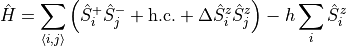
$\hat{H} = \sum_{\langle i,j \rangle} \left(\hat{S}_i^ + \hat{S}_j^- + \mathrm{h.c.} + \Delta \hat{S}^z_i \hat{S}^z_j \right)- h \sum_i \hat{S}^z_i$

over the anisotropy $\Delta$ and the magnetic field $h$ . One begins by building a template dictionary parameters_template for the simulations which includes all information except for the specification for $\Delta$ and $h$ as discussed in Sec. Specifying the parameters of a simulation. The specification of the parameters $\Delta$ and $h$ comes through two lists. The first, called iterparams, is a list of the tags of the Hamiltonian parameters to be parallelized over. The second, called iters, is a list whose elements are a list of the numerical values for the corresponding parameters in iterparams. For our example of the XXZ model, these two vectors might be specified as

Deltamin = 0.1
Deltamax = 2.0
Deltavals = 50
Deltaiter = np.linspace(Deltamin, Deltamax, Deltavals)

hmin = 0.0
hmax = 1.0
hvals = 20
hiter = np.linspace(hmin, hmax, hvals)

iterparams = ['Delta', 'h']
iters = [Deltaiter, hiter]

This would parallelize over the 50 values of $\Delta$ linearly spaced from 0.1 to 2 and the 20 values of $h$ linearly spaced from 0 to 1 for a total of 1000 points. Note that the tags we use here in iterparams should match those we use in building the Hamiltonian MPO, see Sec. Defining the Hamiltonian and other many-body operators. These lists, along with the template dictionary of other metadata, are passed to the function Paralleltools.WriteMPSParallelTemplate(), with syntax

parameters = mps.WriteMPSParallelTemplate(parameters_template, Operators, H, comp_info, iterparams, iters)

Here, comp_info is a dictionary specifying metadata related to the parallel environment. The function Paralleltools.WriteMPSParallelTemplate() writes the files required by the Fortran backend for each individual simulation as well as two files *jobpool.dat and *progress, where * is the 'job\_ID' specified in the parameters_template dictionary. The jobpool file contains the main files which specify the individual simulations to be run together with unique integer tags, and the progress file indicates which of these tasks has already been completed. Finally, Paralleltools.WriteMPSParallelTemplate() writes a pbs or slurm script which will submit a parallel job to your computer’s queueing system. If a job does not finish all of the tasks in the jobpool, calling Paralleltools.WriteMPSParallelTemplate() will create a new job pool containing only simulations which have not been run previously.

An alternate functionality of the parallel code is to pass in a list of parameters to parameters_template.

Paralleltools.WriteMPSParallelTemplate() will automatically parallelize over all of the simulations in parameters_template. A list of Hamiltonians may also be passed to H, but the length of H and parameters_template must be the same. Finally, the two functionalities may be combined by specifying both a list of parameters_template as well as parameters to iterate over via iterparams and iters.

Putting it all together¶

In this section we will analyze the simplest example file given in the Examples subdirectory of OSMPS, 04_SpinlessFermions.py. The file begins by importing MPSPyLib, NumPy, and the module sys

import MPSPyLib as mps
import numpy as np
import sys

Inside the function main we start building the spinless operators

    # Build operators

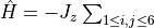
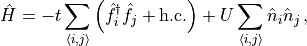
Now, Operators contains the fermion operators given in the table of Ops.BuildFermiOperators(). We now build the Hamiltonian which consists only of tunneling,

(2)¶ $\hat{H}&=-t\sum_{\langle i,j\rangle}\left[\hat{f}_i^{\dagger}\hat{f}_j+\mathrm{h.c.}\right]\, .$

This is done as

    # Define Hamiltonian MPO
    H = mps.MPO(Operators)

The specification 'bond' denotes the sum over nearest-neighbors in Eq. (2) and Phase=True denotes that a Fermi phase should be included, as this term involves an odd number of fermion operators at each site, see Sec. Defining the Hamiltonian and other many-body operators. We next define the observables we wish to measure

    # Observables
    myObservables = mps.Observables(Operators)
    # Correlation functions
    myObservables.AddObservable('corr', ['fdagger','f'], 'bspdm')

Here, the observable we have called 'spdm' is the fermionic single-particle density matrix, $\langle \hat{f}_i^{\dagger}\hat{f}_j \rangle$ , and the observable we have called 'bspdm' is a single-particle density matrix $\langle \hat{\tilde{f}}_i^{\dagger}\hat{\tilde{f}}_j \rangle$ in which the operators $\hat{\tilde{f}}_i$ anticommute on a given site but commute when not on the same site. The difference is in including Phase=True in the observable specification. We will see the differences in the two correlation functions when we run the simulation. Next, we specify the convergence criteria for our simulation as

    # Convergence data

Now, we specify the simulation parameters as

    t = 1.0
    L = 10
    N = 5

    # Define statics
    parameters = [{ 
        # Directories
        'simtype'                   : 'Finite',
        'job_ID'                    : 'SpinlessFermions_',
        'unique_ID'                 : 'L_' + str(L) + 'N' + str(N),
        'Write_Directory'           : 'TMP_04/',
        'Output_Directory'          : 'OUTPUTS_04/',
        # System size and Hamiltonian parameters
        'L'                         : L,
        't'                         : t, 
        'verbose'                   : 2,
        'logfile'                   : True,
        # Specification of symmetries and good quantum numbers
        'Abelian_generators'        : ['nftotal'],
        'Abelian_quantum_numbers'   : [N],

L is the number of lattice sites and t is the tunneling energy. Note that it is only in the dictionary parameters that we specify a value for t; we do not need to give an actual value for t when we are building the Hamiltonian. The lines

        'verbose'                   : 2,
        'logfile'                   : True,

specify that the total number of fermions is conserved, and is set to be N. We write Fortran-readable files and run them with the lines if we are not in the post processing mode:

        'MPSConvergenceParameters'  : myConv
    }]

    # Write Fortran-readable main files
    MainFiles = mps.WriteFiles(parameters, Operators, H,
                               PostProcess=PostProcess)

The observables are read in using

    if(not PostProcess):
        if os.path.isfile('./Execute_MPSMain'):
            RunDir = './'
        else:

Because we have only a single simulation in this case, corresponding to the ground state with a single set of convergence parameters, the relevant outputs are contained in Outputs[0], the first element of the list Outputs, see Sec. Defining and reading observables: obsterms.Observables. The $L\times L$ matrix representing the single-particle density matrix is Outputs[0]['spdm'], as we specified the tag 'spdm' for this observable in line 14. We now diagonalize the single-particle density matrix and its phaseless counterpart 'bspdm' to find their eigenvalues using the numpy function eigh and print the eigenvalues to the screen with

        mps.runMPS(MainFiles, RunDir=RunDir)
        return

    # Postprocessing
    # --------------

    Outputs = mps.ReadStaticObservables(parameters)

    spdm = Outputs[0]['spdm']

The return state indicates the end of the main function. The last lines call our main function in the case the file is call from command line and handle the post processing argument from the command line. If it was included as module the main function would not be executed.

    bspdmeigs, U = np.linalg.eigh(bspdm)

    print('Eigenvalues of <f^{\dagger}_i f_j> with Fermi phases', spdmeigs)
    print('Eigenvalues of <f^{\dagger}_i f_j> without Fermi phases', bspdmeigs)

    return

if(__name__ == '__main__'):

Calling

osmps@manual:~$ python 04_SpinlessFermions.py

in the terminal gives the output

./Execute_MPSMain TMP/SpinlessFermions_L_10N5Main.nml
Eigenvalues of <f^{\dagger}_i f_j> with Fermi phases [ -4.56780243e-16  -4.34812894e-17   2.50202620e-16
   5.99741719e-13 6.00558567e-13   1.00000000e+00   1.00000000e+00   1.00000000e+00
   1.00000000e+00   1.00000000e+00]
Eigenvalues of <f^{\dagger}_i f_j> without Fermi phases [ 0.05067985  0.06159355  0.09456777  0.12959356
  0.17094556  0.35616646 0.45241313  0.60737271  0.91929511  2.1573723 ]

We see that the properly phased single-particle density matrix produces a sharp Fermi distribution, as expected. Contrariwise, the single-particle density matrix without the Fermi phases displays a macroscopically large eigenvalue.

Footnotes

Simulation Details¶

Including the required Python libraries¶

Specifying the parameters of a simulation¶

Defining local operators¶

Overview of operators in MPSPyLib¶

Operators with internal degrees of freedom¶

Defining the Hamiltonian and other many-body operators¶

Matrix Product Operators¶

MPO Terms to build rule sets¶

Defining and reading observables: `obsterms.Observables`¶

Defining Observables¶

Reading Observables¶

Specification of dynamics¶

Abelian symmetries¶

Convergence criteria¶

Running simulations¶

Running a serial static simulation¶

Running a parallel static simulation¶

Parallel simulations via a list¶

Parallel simulations via a template¶

Putting it all together¶

Table of Contents

Previous topic

Next topic

This Page

Simulation Details¶

Including the required Python libraries¶

Specifying the parameters of a simulation¶

Defining local operators¶

Overview of operators in MPSPyLib¶

Operators with internal degrees of freedom¶

Defining the Hamiltonian and other many-body operators¶

Matrix Product Operators¶

MPO Terms to build rule sets¶

Defining and reading observables: obsterms.Observables¶

Defining Observables¶

Reading Observables¶

Specification of dynamics¶

Abelian symmetries¶

Convergence criteria¶

Running simulations¶

Running a serial static simulation¶

Running a parallel static simulation¶

Parallel simulations via a list¶

Parallel simulations via a template¶

Putting it all together¶

Defining and reading observables: `obsterms.Observables`¶