Algorithms of the OpenMPS
In this section we provide some details on the algorithms used by OSMPS in order to give the user some understanding of the available convergence parameters. The reader interested in a broader view of MPSs and their algorithms should consult Ulrich Schollwoeck’s review The density-matrix renormalization group in the age of matrix product states, which is the standard reference on the subject at the time of writing of this manual [Schollwock11].
Definitions
We define a tensor as a map from a product of Hilbert spaces to the complex numbers

Here  is the rank of the tensor. If we evaluate the elements of the
tensor
is the rank of the tensor. If we evaluate the elements of the
tensor  in a fixed basis
  for each
Hilbert space
for each
Hilbert space  , then equivalent information is carried in
the multidimensional array
, then equivalent information is carried in
the multidimensional array  . We will also refer to
this multidimensional array as a tensor. The information carried in a tensor
does not change if we change the order in which its indices appear. We will
call such a generalized transposition a permutation of the tensor. As an
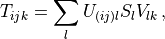
example, the permutations of the rank-3 tensor are
. We will also refer to
this multidimensional array as a tensor. The information carried in a tensor
does not change if we change the order in which its indices appear. We will
call such a generalized transposition a permutation of the tensor. As an
example, the permutations of the rank-3 tensor are
![T_{ijk}&=\left[T'\right]_{kij}=\left[T''\right]_{jki}=\left[T'''\right]_{jik}=\left[T''''\right]_{kji}=\left[T'''''\right]_{ikj}\, .](../_images/math/9747ec4a32731982578d5c46656100d3a39905bf.png)
Here, the primes indicate that the tensor differs from its unprimed counterpart
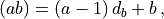
only by a permutation of indices. Similarly, by combining two such indices
together using the Kronecker product we can define an equivalent tensor of
lower rank, a process we call index fusion. We denote the Kronecker product
of two indices  and
and  using parentheses as
 , and a representation is provided by
where  is the dimension of
  and and
are both indexed starting from 1. An example of fusion is
and and
are both indexed starting from 1. An example of fusion is
![T_{ijk}&=\left[T'\right]_{i\left(jk\right)}\, .](../_images/math/5aa6ddf33040e7de56cab672c565f3c19ed5f223.png)
Here, is a rank-3 tensor of dimension  and
and  is a matrix of dimension
  . The inverse
operation of fusion, which involves creating a tensor of higher rank by
splitting a composite index, we refer to as index splitting.
. The inverse
operation of fusion, which involves creating a tensor of higher rank by
splitting a composite index, we refer to as index splitting.
Just as permutations generalize the notion of matrix transposition,
tensor contraction generalizes the notion of matrix multiplication. In a
contraction of two tensors A and B some set of indices  and
and  which describe a common Hilbert space are summed,
and the resulting tensor
which describe a common Hilbert space are summed,
and the resulting tensor  consists of products of the elements of
 and
and  as
as
(7)
Here  denotes the indices of which are not
contracted and likewise for . The rank of
is
denotes the indices of which are not
contracted and likewise for . The rank of
is  , where
  is the number of indices contracted
(i.e., the number of indices in
is the number of indices contracted
(i.e., the number of indices in  ) and
) and  and
and
 are the ranks of and , respectively. In writing
expression Eq. (7) we have permuted all of the indices
to be contracted to the furthest right position in
and the indices to the furthest leftmost
position in for notational simplicity.
are the ranks of and , respectively. In writing
expression Eq. (7) we have permuted all of the indices
to be contracted to the furthest right position in
and the indices to the furthest leftmost
position in for notational simplicity.
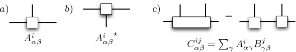
Fig. 1 Examples of basic tensor operations in diagrammatic notation. a) A rank-3 tensor. b) The conjugate of a rank-3 tensor. c) The contraction of two rank-3 tensors over a single index produces a rank-4 tensor.
At this stage, it is advantageous to develop a graphical notation for tensors and their operations [SDV06]. A tensor is represented graphically by a box with lines extending upwards from it. The number of lines is equal to the rank of the tensor. The order of the indices from left to right is the same as the ordering of lines from left to right. A contraction of two tensors is represented by a line connecting two points. Finally, the complex conjugate of a tensor is denoted by a point with lines extending downwards. Some basic tensor operations are shown in graphical notation in Fig. 1.
Following a similar line of reasoning as for contractions above, we may also
decompose tensors into contractions of tensors using permutation, fusion,
and any of the well-known matrix decompositions such as the singular value
decomposition (SVD) or the QR decomposition. For example, a rank-3 tensor
can be factorized as
where  and
and  are unitary and
  is a positive
semidefinite real vector. Such decompositions are of great use in MPS
algorithms.
is a positive
semidefinite real vector. Such decompositions are of great use in MPS
algorithms.
A tensor network is now defined as a set of tensors whose indices are
connected in a network pattern, see Fig. 2. Let us consider that some
set of the network’s indices are contracted over, and the
complement  remain uncontracted. Then, this network
is a decomposition of some tensor
remain uncontracted. Then, this network
is a decomposition of some tensor  . The basic
idea of tensor network algorithms utilizing MPSs and their higher dimensional
generalizations such as projected entangled-pair states
(PEPS) [VC04], [VMC08] and the multiscale
entanglement renormalization algorithm (MERA) [Vid07], [EV09]
are to represent the high-rank tensor
. The basic
idea of tensor network algorithms utilizing MPSs and their higher dimensional
generalizations such as projected entangled-pair states
(PEPS) [VC04], [VMC08] and the multiscale
entanglement renormalization algorithm (MERA) [Vid07], [EV09]
are to represent the high-rank tensor  encoding a
many-body wavefunction in a Fock basis,
encoding a
many-body wavefunction in a Fock basis,
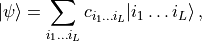
as a tensor network with tensors of small rank. We set the convention that indices which are contracted over in the tensor network decomposition will be denoted by Greek indices, and indices which are left uncontracted will be denoted by Roman indices. The former type of index will be referred to as a bond index, and the latter as a physical index.
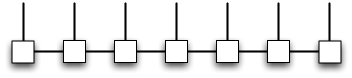
Fig. 2 An MPS with 7 sites and open boundary conditions.
In particular, an MPS imposes a one-dimensional topology on the tensor network such that all the tensors appearing in the decomposition are rank-3. The resulting decomposition has the structure shown in Fig. 2. Explicitly, an MPS may be written in the form
(8)¶![|\psi_{\mathrm{MPS}}\rangle=\sum_{i_1,\dots i_L=1}^{d}\mathrm{Tr}\left(A^{\left[1\right]i_1}\dots A^{\left[L\right]i_L}\right)|i_1\dots i_L\rangle\, .](../_images/math/55e5dad19a583a91107a6029e6b87607d7ae5924.png)
Here,  label the
  distinct sites, each of which
contains a
distinct sites, each of which
contains a  dimensional Hilbert space. We will call the
local dimension. The superscript index in brackets
dimensional Hilbert space. We will call the
local dimension. The superscript index in brackets ![\left[j\right]](../_images/math/15012fee03510d702d94ca63087f0e1c0576d38d.png) denotes that this is the tensor of the
denotes that this is the tensor of the  site, as these
tensors are not all the same in general. Finally, the trace effectively sums
over the first and last dimensions of
site, as these
tensors are not all the same in general. Finally, the trace effectively sums
over the first and last dimensions of ![A^{\left[1\right]i_1}](../_images/math/01e09c0885e58d3a80259c6fd781ed367905a696.png) and
and
![A^{\left[L\right]i_L}](../_images/math/0c87dff757c77beb59df509234ecc2bd894c5a7d.png) concurrently, and is necessary only for periodic
boundary conditions where these dimensions are greater than 1. All algorithms
in OSMPS work only with open boundary conditions. Obscured within the matrix
product of Eq. (8) is the size of the matrix
concurrently, and is necessary only for periodic
boundary conditions where these dimensions are greater than 1. All algorithms
in OSMPS work only with open boundary conditions. Obscured within the matrix
product of Eq. (8) is the size of the matrix
![A^{\left[j\right]i_j}](../_images/math/3fdf8a5dcad160c98d80459300e83a0dcf8b14ac.png) formed from the tensor
formed from the tensor ![A^{\left[j\right]}](../_images/math/3d4ed1850293cc75a4512d4821d6c495551a18a0.png) with its physical index held constant. We will refer to the left and right
dimensions of this matrix as
with its physical index held constant. We will refer to the left and right
dimensions of this matrix as  and
and  , and the
maximum value of
, and the
maximum value of  for any tensor, the bond dimension, will be
denoted as
for any tensor, the bond dimension, will be
denoted as  . The bond dimension is the parameter which determines
the efficiency of an MPS simulation, and also its dominant computational
scaling. From the relation
. The bond dimension is the parameter which determines
the efficiency of an MPS simulation, and also its dominant computational
scaling. From the relation  , where
 is the maximum von Neumann entropy of entanglement of
any bipartite splitting, we also have that represents an
entanglement cutoff for MPSs.
is the maximum von Neumann entropy of entanglement of
any bipartite splitting, we also have that represents an
entanglement cutoff for MPSs.
Variational ground state search
OSMPS implements the two-site variational ground state search algorithm. In this algorithm, the state which minimizes the energy globally is sought by minimizing the energy of the state with all but two contiguous sites held fixed. The position of the two variational sites is then moved throughout the lattice as in Fig. 3.
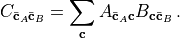
The local minimization begins by fusing the MPS tensors of the two sites to be optimized together to create a rank four tensor,
![\Theta_{\alpha\beta}^{ij}&=\sum_{\gamma}A^{\left[k\right] i}_{\alpha \gamma}A^{\left[k+1\right]j}_{\gamma\beta}\, .](../_images/math/17b19fdbf1772b41e10347f712e5fcd749219eed.png)
The Hamiltonian is then projected onto the Hilbert space of  by
fixing all other MPS tensors, resulting in the effective Hamiltonian
by
fixing all other MPS tensors, resulting in the effective Hamiltonian
 . The energy is then minimized locally by solving
the effective Hamiltonian eigenvalue problem
. The energy is then minimized locally by solving
the effective Hamiltonian eigenvalue problem

for the lowest energy eigenpair  . The effective
linear dimension of is very large, but this
matrix is also sparse in typical situations. Hence, we use a sparse iterative
eigenvalue solver, the Lanczos algorithm, to determine the eigenpair
corresponding to the lowest energy. In this algorithm there are two
convergence parameters, The first is
. The effective
linear dimension of is very large, but this
matrix is also sparse in typical situations. Hence, we use a sparse iterative
eigenvalue solver, the Lanczos algorithm, to determine the eigenpair
corresponding to the lowest energy. In this algorithm there are two
convergence parameters, The first is  , the number of
iterations which are allowed before the algorithm claims to have not converged.
The second is a stopping tolerance
, the number of
iterations which are allowed before the algorithm claims to have not converged.
The second is a stopping tolerance  on an
eigenpair which is determined by the residual
on an
eigenpair which is determined by the residual
After the local minimization has been performed, we must return the state to
its canonical MPS decomposition. We do so by decomposing into
two rank three tensors
![\sum_{\gamma}A^{\left[k\right] i}_{\alpha \gamma}A^{\left[k+1\right]j}_{\gamma\beta}&=\Theta_{\alpha\beta}^{ij}\, .](../_images/math/7421e4b42377a12fb31f218de8749d548e1a9f29.png)
This decomposition may involve a truncation of the bond dimension, which here
would be the dimension of the space indexed by  . In OSMPS, this
dimension is determined implicitly by
. In OSMPS, this
dimension is determined implicitly by
(9)
where  is the vector of singular values of the matrix
epsilon_{mathrm{local}} is a user-supplied local tolerance, and we will
call  the local truncation error. The user may also
specify a maximum bond dimension
the local truncation error. The user may also
specify a maximum bond dimension  which takes
precedence over the condition Eq. (9). The complete sequence of
local minimization is shown in the blue box in Fig. 3.
which takes
precedence over the condition Eq. (9). The complete sequence of
local minimization is shown in the blue box in Fig. 3.
After the minimization of two sites with indices  and
and
 , we minimize the sites and
  and continue optimizing pairs of sites further to the right until we reach the
right boundary. At the right boundary, we reverse direction and optimize pairs
of sites with decreasing indices until we reach the left boundary. Here, we
again reverse direction and optimize pairs of sites until we reach the pair of
sites and again. We have now completed an
inner sweep in which each pair of contiguous sites has been optimized twice.
Convergence of the variational state to the ground state is ascertained by the
variance condition
and continue optimizing pairs of sites further to the right until we reach the
right boundary. At the right boundary, we reverse direction and optimize pairs
of sites with decreasing indices until we reach the left boundary. Here, we
again reverse direction and optimize pairs of sites until we reach the pair of
sites and again. We have now completed an
inner sweep in which each pair of contiguous sites has been optimized twice.
Convergence of the variational state to the ground state is ascertained by the
variance condition
If convergence is achieved, the program exits, otherwise another inner sweep
is performed. If convergence is not reached when the maximum number of inner
sweeps has been reached, then the program tries to decrease the local tolerance
to meet the desired variance tolerance by assuming that the variance is
proportional to the site-integrated local truncation error and performing
linear extrapolation. The inner sweeping procedure is then repeated. We call
such an iteration an outer sweep. The convergence parameters for this
algorithm are set by an object of the convergence.MPSConvParam
class. In particular, the relevant parameters and their default values are
collected in the table convergence.MPSConvParam.
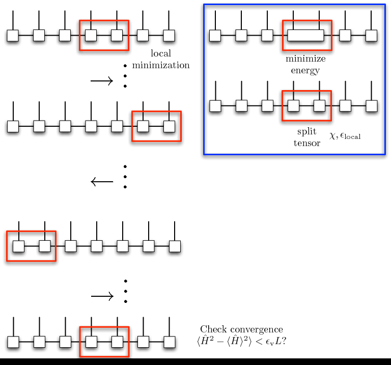
Fig. 3 Variational ground state search on 7 sites. The energy of the two sites
enclosed in the red box is locally minimized by solving the effective
Hamiltonian eigenproblem with the Lanczos iteration. The associated
two-site eigenvector is then decomposed to maintain a consistent MPS
canonical form with local tolerance  and
maximum bond dimension as shown in the blue box. The position
of the two sites being minimized is moved throughout the entire lattice in
a sweeping motion. After each pair of sites has been optimized twice,
convergence is checked by considering whether the variance meets the
desired tolerance.
and
maximum bond dimension as shown in the blue box. The position
of the two sites being minimized is moved throughout the entire lattice in
a sweeping motion. After each pair of sites has been optimized twice,
convergence is checked by considering whether the variance meets the
desired tolerance.
Variational excited state search: eMPS
The algorithm for finding excited states variationally with MPSs, which we
call eMPS [WC12], uses a process of local minimization and
sweeping similar to the variational ground state search. The difference is
that the the local minimization is performed using a projected effective
Hamiltonian which projects the variational state into the space orthogonal to
all other previously obtained eigenstates. Hence, the convergence parameters
which are used for eMPS are identical to those used for the variational ground
state search collected in the table of convergence.MPSConvParam.
The eMPS method is used whenever the key 'n_excited_states' in
parameters has a value greater than zero, see Sec. Specifying the parameters of a simulation.
iMPS as initial ansatz
As the MPS methods used in OSMPS are variational, their efficiency is greatly enhanced by the availability of a good initial guess for the wavefunction. For the ground state, a good guess can be found by using a fixed number of iterations of the infinite size variational ground state search with MPSs (iMPS) to be discussed in more detail in Sec. Infinite-size ground state search: iMPS. In this method, we begin by considering two sites and minimize the energy locally using the Lanczos iteration as discussed in Sec. Variational ground state search. We then decompose the two-site wavefunction into two separate rank three tensors and then use these tensors as an effective environment into which two new sites are embedded as in Fig. 4. The energy of these two inner sites is minimized with the environment sites held fixed, and then these sites are absorbed into the environment and a new pair 1 of sites is inserted into the center. This process is repeated until we have a chain of sites which has the desired length. We call this process the warmup phase.
The parameters used to control the convergence of the warmup phase are
included as part of the convergence.MPSConvParam class. In
addition to the Lanczos convergence parameters discussed in
Sec. Variational ground state search and the table in convergence.MPSConvParam, the
warmup-specific parameters are  , the maximum bond
dimension allowed during warmup and
, the maximum bond
dimension allowed during warmup and  , the local
truncation determining the bond dimension according to Eq. (9)
during warmup. These convergence parameters are set in an object of the
, the local
truncation determining the bond dimension according to Eq. (9)
during warmup. These convergence parameters are set in an object of the
convergence.MPSConvParam class as specfied in the table in its
class documentation. Note that only the values of the warmup
convergence parameters from the first set of convergence parameters are used.
That is to say, warmup is only used to construct an initial state, and
subsequent refinements use the output from variational ground state search as
the input to a more refined variational ground state search. Also note that
warmup is only relevant to ground state search and not excited state search,
and so setting values of the warmup convergence parameters for objects of the
convergence.MPSConvParam class to be used for eMPS has no
effect.
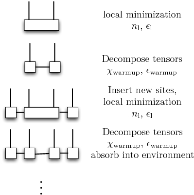
Fig. 4 The iMPS iteration successively adds sites to the center of a chain, performs local minimization of the energy with only these sites, and then absorbs these sites into the environment.
- 1
For finite lattices with an odd number of sites, a single site is inserted on the last iteration.
Infinite-size ground state search: iMPS
In addition to being used to initialize finite-size simulations, a variation
of the iMPS method presented in Sec. iMPS as initial ansatz can also be used
to find a representation of an infinitely large wavefunction which is
translationally invariant under shifts by some number of sites  .
The convergence behavior of iMPS is determined by an object of the
.
The convergence behavior of iMPS is determined by an object of the
convergence.iMPSConvParam class. The iMPS minimization is
performed by inserting sites at each iMPS iteration as shown in
Fig. 4 and then minimizing the energy of these sites
with the given fixed environment. After minimization, these sites are absorbed
into the environment, new sites are added, and the minimization is
repeated. The iteration has converged when two unit cells are close in some
sense. This sense is measured rigorously by the orthogonality
fidelity [McCulloch08]. In OSMPS, we take the stopping condition to be
that the orthogonality fidelity is less than the unit-cell averaged truncation
error as measured by Eq. (9) for 10 successive iterations. If
there is no truncation error, then the stopping criterion is that the
orthogonality fidelity is less than  for 10
successive iterations, where is the
for 10
successive iterations, where is the
'variance_tol' in tools.MPSConvergenceParameters. This
convergence condition on the orthogonality fidelity denotes that the
differences between successive iterations are due only to truncation arising
from a finite bond dimension. A maximum number of iterations may also be
specified as 'max_num_imps_iter'.
The variance is not used to determined convergence of a unit cell to its
minimum. Rather, a fixed number of sweeps, specified by 'min_num_sweeps'
are used to converge. Hence, the relevant convergence parameters for an iMPS
simulation are the parameters of convergence.iMPSConvParam
collected in Table in convergence.iMPSConvParam.
Krylov-based time evolution : tMPS
The Krylov-based tMPS algorithm [WC12] has its own class of
convergence parameters called convergence.KrylovConvParam.
Its parameters are collected in the class description. While many of these
parameters have the same names as those in
convergence.MPSConvParam they have different interpretations.
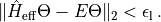
The Lanczos procedure now refers to the Lanczos method for determining the
matrix exponential, and so the stopping criterion is that the difference
between our variational state and the true state acted on by the matrix
exponential is less than 'lanczos_tol' in the 2-norm. The action of an
operator  on a state
  and the representation
of a sum
and the representation
of a sum  cannot be represented exactly as MPSs
for a given fixed bond dimension, and so both of these operations are performed
with variational algorithms as discussed in Ref. [WC12]. The
associated convergence parameters for these two variational algorithms are given
in the functions description at
cannot be represented exactly as MPSs
for a given fixed bond dimension, and so both of these operations are performed
with variational algorithms as discussed in Ref. [WC12]. The
associated convergence parameters for these two variational algorithms are given
in the functions description at convergence.KrylovConvParam as well.
Time Evolving Block Decimbation (TEBD)
The TEBD algorithm uses the Sornborger-Stewart decomposition
[SS99] instead of the more common Trotter decomposition. As
for the Trotter decomposition, this method is only valid for nearest-neighbor
Hamiltonians built from site and bond rules. At present, it uses the Krylov
subspace method to apply the exponential of the two-site Hamiltonian to the
state. The convergence parameters are described in details in
convergence.TEBDConvParam.
Time-Dependent Variational Principle (TDVP)
The Time-Dependent Variational Principle is the second algorithm after
Krylov to support long-range interactions represented in the MPO. Its
convergence parameters are specified in convergence.TDVPConvParam.
Details on the algorithm can be found in [HLO+16].
Local Runge-Kutta (LRK)
The Local Runge-Kutta algorithm [ZMK+15] generates a MPO
representation of the propagator which can be applied to the state. The
details on the convergence parameters are in
convergence.LRKConvParam.