Python Module mpo¶

Matrix Product Operators¶

The matrix product operators organize the class mpo.MPO. The natural operator structure for MPS algorithms is a matrix product operator (MPO). The exact diagonalization modules uses the same class to construct Hamiltonians, effective Hamiltonians, and operators in Liouville space. Operators can be constructed as MPOs using a set of rules which specify how operators acting on local Hilbert spaces are combined to create an operator acting on the entire many-body system. Using a canonical form for MPOs, several operators constructed from these rules can be put together as a single MPO [WC12]. OSMPS uses this essential idea of creating operators from a set of predetermined rules to construct the Hamiltonian and other operators appearing in an MPS simulation.

An operator acting on the many-body state, i.e. the MPO, is an object of the mpo.MPO class in MPSPyLib. For an instantiation of the MPO class, named H in the following, is obtained as

H = mps.MPO(Operators)

Once we have an MPO object, we add terms to it using the Ops.AddMPOTerm() method. In particular, the rules are defined in the module mpoterm.

MPO Terms to build rule sets¶

The following MPO terms are available at present

site rule (mpoterm.SiteTerm). Example:

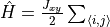
H.AddMPOTerm('site', 'sz', hparam='h_z', weight=1.0)
generates $\hat{H}=h_z\sum_{i=1}^{L}\hat{S}^z_i$ , where $\hat{S}^z =$ Operators['sz']} and Operators was already passed when creating the instance of the MPO. The second argument contains the relevant keys of the operators to be used. Because only the names of the operators are used, this routine handles ordinary and symmetry-adapted operators on the same footing.

bond rule (mpoterm.BondTerm). Example:

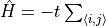
H.AddMPOTerm('bond', ['splus','sminus'], hparam='J_xy', weight=0.5)
generates $\hat{H} = \frac{J_{xy}}{2} \sum_{\langle i,j \rangle}$ $\left(\hat{S}^{+}_{i} \hat{S}^{-}_{j} + \mathrm{h.c.} \right)$ , where $\langle i,j\rangle$ denotes all nearest neighbor pairs $i$ and $j$ ,
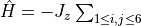
H.AddMPOTerm('bond', ['sz', 'sz'], hparam='J_z', weight=1.0)
generates $\hat{H}=J_{z}\sum_{\langle i,j\rangle}\hat{S}^z_i\hat{S}^z_j$ , and
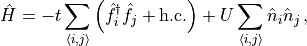
H.AddMPOTerm('bond', ['fdagger', 'f'], hparam='t', weight=-1.0, Phase=True)
generates $\hat{H} = -t \sum_{\langle i,j \rangle}$ $\left(\hat{f}_i^{\dagger} \hat{f}_j + \mathrm{h.c.} \right)$ , where $\hat{f}$ is a fermionic destruction operator. That is, terms with Fermi phases are cared for with the optional Phase argument and Hermiticity is automatically enforced by this routine. The Fermi phase is added through a Jordan-Wigner string of the operators in Operator with key FermiPhase. The functions Ops.BuildFermiOperators() and Ops.BuildFermiBoseOperators() discussed in Sec. Defining local operators both create the Fermi phase operator appropriate for this use automatically. Notice that the order of the operators matters due to the Jordan-Wigner transformation. Adding ['f', 'fdagger'] does not result in the same fermionic Hamiltonian. A warning will be printed for obvious cases.

exponential rule set (mpoterm.ExpTerm). Example

H.AddMPOTerm('exponential', ['sz', 'sz'], hparam='J_z', decayparam=a, weight=1.0)
generates $\hat{H} =J_z \sum_{i<j} a^{j-i+1} \hat{S}^z_i \hat{S}^z_j$ . This rule also enforces Hermiticity and cares for Fermi phases as in the bond rule case.

FiniteFunction rule (mpoterm.FiniteFunc). Example:

f = []
for ii in range(6):
    f.append(1.0 / (ii + 1.0)**3)
H.AddMPOTerm('FiniteFunction', ['sz', 'sz'], f=f, hparam='J_z', weight=-1.0)
generates $\hat{H} = -J_z \sum_{1 \le i,j \le 6}$ $\frac{1}{\left|j-i \right|^3} \hat{S}^z_i \hat{S}^z_j$ , where the summation is over all $i$ and $j$ pairs separated by at least $1$ and at most $6$ lattice spacings. The range of the potential is given by the number of elements in the list f. This rule enforces Hermiticity and cares for Fermi phases as in the bond rule case.

InfiniteFunction rule set (mpoterm.InfiniteFunc). We point out that this term is always fitted with a set of mpoterm.ExpTerm for MPS simulations. Examples:

invrcube = lambda x: 1.0/(x*x*x)
H.AddMPOTerm('InfiniteFunction', ['sz', 'sz'], hparam='J_z', weight=1.0,
             func=invrcube, L=1000, tol=1e-9)
generates $\hat{H}=\sum_{i<j}\frac{1}{\left|j-i\right|^3}\hat{S}^z_i\hat{S}^z_j$ , where the functional form is valid to a distance L with a residual of at most tol. Similarly,
H.AddMPOTerm('InfiniteFunction', ['sz', 'sz'], hparam='J_z', weight=1.0, 
             x=x, y=f, tol=1e-9)
generates $\hat{H}=\sum_{i<j}f\left(j-i\right)\hat{S}^z_i\hat{S}^z_j$ , where the functional form $f\left(x\right)$ is determined by the array of values f and the array of evaluation points x. The distance of validity L is determined from the array x. This rule applies only to monotonically decreasing functions func or f, and so outside the range of validity L the corrections are also monotonically decreasing. This rule enforces Hermiticity and cares for Fermi phases as in the bond rule case.

product rule (mpoterm.ProductTerm). Example:

H.AddMPOTerm('product', 'sz', hparam='h_p', weight=-1.0)
generates $\hat{H}=-h_p\prod_{i=1}^{L} \hat{S}^z_i$ . The operator used in the product must be Hermitian.

MBString rule set(mpoterm.MBStringTerm). See function description for usage.
mpoterm.TTerm. See function description for usage.
mpoterm.SiteLindXX. See function description for usage.
mpoterm.LindExp. See function description for usage.
mpoterm.LindInfFunc. See function description for usage.
mpoterm.MBSLind. See function description for usage. (Can act as nearest neighbor Lindblad term.)

In all of the above expressions, H is an object of the MPO class. The strings passed to the argument hparams represent tags for variable Hamiltonian parameters, which allow for easy batching and parallelization (Sec. Running a parallel static simulation), and also facilitate dynamical processes The argument hparams is optional, and defaults to the constant value 1. The optional argument weight specifies a constant factor that scales the operator and defaults to the value 1, too.

Developer’s Guide for Rule Sets

Module contains a class for each possible term in the MPO rule sets. Each term is derived from a base class.If you plan to add additional MPO terms to OSMPS, you have to modify the following files. In the case of a new Lindblad operator, these are

mpoterm.py: add class for the new term
mpo.py: add new term to the MPO structure and enable writing.
MPOOps_types_templates.f90: define derived type and add to MPORuleSet
MPOOps_include.f90: add read/destroy methods for RuleSets
MPOOps_include.f90: effective Hamiltonian for 2 sites
MPOOps_include.f90: Liouville operator for 2 sites
MPOOps_include.f90: effective Hamiltonian represented as MPO.
MPOOps_include.f90: Liouville operator represented as MPO.
TimeevolutionOps_include.f90: Add overlaps to QT functionality.

Example

As an example, a template MPO for the Hamiltonian of the hard-core boson model with $1/r^3$ interactions,

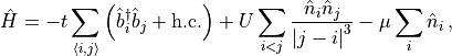
$\hat{H} &= -t \sum_{\langle i,j \rangle} \left(\hat{b}_i^{\dagger} \hat{b}_j + \mathrm{h.c.} \right) + U \sum_{i<j} \frac{\hat{n}_i \hat{n}_j}{\left|j-i \right|^3} - \mu \sum_{i} \hat{n}_i \, ,$

is provided by

import MPSPyLib as mps

# Build operators
Operators = mps.BuildBoseOperators(1)
# Define Hamiltonian MPO
H = mps.MPO(Operators)
H.AddMPOTerm('site', 'nbtotal', hparam='mu', weight=-1.0)
H.AddMPOTerm('bond', ['bdagger', 'b'], hparam='t', weight=-1.0)
invrcube = lambda x: 1.0/(x*x*x)
H.AddMPOTerm('InfiniteFunction', ['nbtotal', 'nbtotal'], hparam='U',
             weight=1.0, func=invrcube, L=1000, tol=1e-9)

We stress that no assumptions are made about the hparam parameters 't', 'mu', or 'U' when the MPO is built. The hparams are simply tags parameterizing the operators which appear in the Hamiltonian. The actual numerical values of $t$ , $U$ , and $\mu$ are specified as part of the dictionary parameters discussed in Sec. Specifying the parameters of a simulation. These parameters can also be position-dependent, as demonstrated in the example files in OpenMPS Examples.

One can print operators using the mpo.MPO.printMPO() method. As an example, the interacting spinless fermion model

$\hat{H} &= - t \sum_{\langle i,j \rangle} \left(\hat{f}_i^{\dagger} \hat{f}_j + \mathrm{h.c.} \right) + U\sum_{\langle i,j \rangle }{\hat{n}_i \hat{n}_j} \, ,$

is specified and printed as

import MPSPyLib as mps

# Build operators
Operators = mps.BuildFermiOperators()
# Define Hamiltonian MPO
H = mps.MPO(Operators)
H.AddMPOTerm('bond', ['fdagger', 'f'], hparam='t', weight=-1.0, Phase=True)
H.AddMPOTerm('bond', ['nftotal', 'nftotal'], hparam='U', weight=1.0)
H.printMPO()

The result of this code is

-1.0 * t * sum_i fdaggerP_i f_{i+1} + 1.0 * t * sum_i fP_i fdaggerP_{i+1} + 1.0 * U * sum_i nftotal_i nftotal_{i+1}

Note the use of the phased operators fdaggerP and fP according to Phase=True.

As the 'InfiniteFunction' rule constructs MPOs by fitting the decaying function to a series of weighted exponentials, the result of printMPO will contain the data for the exponentials and not information about the infinite function proper.

Finally, as complex MPOs with InfiniteFunction interactions can be expensive to generate, one can save the data in an MPO object instance using the mpo.WriteMPO() function, and then read it in later using the mpo.ReadMPO() function. The syntax for these is

mps.WriteMPO(H,filename)
H = mps.ReadMPO(filename)

where H is an object of the mpo.MPO class and filename is the name of the file where the MPO is written to/read from.

mpo.set_interaction_picture(status)[source]¶

mpo.WriteMPO(MPO, filename)[source]¶

Write MPO object instance to file filename.

Arguments

MPOinstance of mpo.MPO: This is the MPO to be written.
filenamestr: File where MPO information is to be written.

mpo.ReadMPO(filename)[source]¶

Read MPO object instance from file filename.

Arguments

filenamestr: Filename where MPO is stored.

class mpo.MPO(Operators, pbc=False, PostProcess=False)[source]¶

Initialize an MPO object.

Arguments

Operatorsdict or instance of Ops.OperatorList.: Contains the local operators used for measurements, symmetries, and MPOs.
pbcboolean: Contains the setting for open boundary conditions (False) versus periodic boundary conditions (True). There are multiple restrictions which methods can be used with PBC. In TN methods, the only non-local terms supporting PBC are the bond rules and the product rule. In ED, only bond rules access the pbc flag, others might execute with OPC. Default to False, i.e., open boundary conditions.
PostProcessboolean, optional: If PostProcessing (True), infinite functions are not fitted with exponentials. If False, those are fitted.

Variables

TIbool: Flag if MPO is translational invariant.
IntHparamdictionary: Contains the mapping string identifier to integer for writting to fortran interface.
termslist: List of available MPO rules.
datadictionary: Contains the class for each rule set with the string identifier as key.

AddMPOTerm(termtype, terms, **kwargs)[source]¶

Add a term to an MPO object

Arguments

termtypestr

Identifies which MPO term should be added. The following options are available: site, bond, FiniteFunction, exponential, product, MBString, InfiniteFunction, and tterm.

termsstr, list of strings

This arguments varies from MPOTerm to MPO term. You can find the explicit description for each term in the corresponding description

mpoterm.SiteTerm
mpoterm.BondTerm
mpoterm.ExpTerm
mpoterm.FiniteFunc
mpoterm.InfiniteFunc
mpoterm.ProductTerm
mpoterm.MBStringTerm
mpoterm.TTerm
mpoterm.SiteLindXX (exact diagonalization)

**kwargsdepends

The optional keyword argument depend as well on the type of the MPO term. See links to descriptions in previous arguments.

IndexHParams()[source]¶: Index the hamiltonian parameters using integers instead of human-readable keys.

_build_effhamiltonian_nosymm(param, sparse, maxdim, quenchtime)[source]¶: Build the effective Hamiltonian describing the hermitian part of the Lindblad master equation. For description of arguments see mpo.MPO.build_effhamiltonian().

_build_effhamiltonian_symm(param, SymmSec, sparse, maxdim, quenchtime, lil=False)[source]¶: Build the effective Hamiltonian decribing the hermitian part of the Lindblad master equation. For description of arguments see mpo.MPO.build_effhamiltonian().

_build_hamiltonian_nosymm(param, sparse, maxdim, quenchtime)[source]¶: Build the Hamiltonian on a complete Hilbert space as sparse/dense matrix. For arguments description look into mpo.MPO.build_hamiltonian().

_build_hamiltonian_symm(param, SymmSec, sparse, maxdim, quenchtime, lil=False)[source]¶: Build a sparse or dense Hamiltonian directly in the symmetry-adapted subspace. For argument description see mpo.MPO.build_hamiltonian().

_build_liouville_nosymm(param, sparse, maxdim, quenchtime)[source]¶: Build the Liouville operator without any symmetry conservation. For arguments look into mpo.MPO.build_liouville().

_build_liouville_symm(param, SymmSec, sparse, maxdim, quenchtime)[source]¶: Build propagator in Liouville space with symmetry. For arguments look into mpo.MPO.build_liouville().

_col_ind_dic(Op)[source]¶

Create a dictionary taking a row index as key and returning the corresponding non-zero elements of the operators as tuple (column index, value).

Arguments

Opnumpy 2d array: Operators to be transfered into this format.

build_effhamiltonian(param, SymmSec, sparse, maxdim, quenchtime)[source]¶

Build the effective Hamiltonian representing the hermitian part of the Lindblad master equation.

Arguments

paramdictionary with simulation parameters: settings of the whole simulation.
SymmSecinstance of SymmmetrySector or None: No meaning here, needed to keep calls equal to sparse equivalent
sparsebool: flag if sparse matrix should be used for Hamiltonian.
maxdimint: limits the dimension of the complete Hilbert space.
quenchtimelist / tuple: If present first entries specifies the number of the quench and second entry the actual time in the whole time evolution. The effective Hamiltonian can only be used in the dynamics, so term has to be present.

build_hamiltonian(param, SymmSec, sparse, maxdim, quenchtime=None)[source]¶

Build the Hamiltonian for the simulation.

Arguments

paramdictionary with simulation parameters: settings of the whole simulation.
SymmSecinstance of SymmmetrySector or None: No meaning here, needed to keep calls equal to sparse equivalent
sparsebool: flag if sparse matrix should be used for Hamiltonian.
maxdimint: limits the dimension of the complete Hilbert space.
quenchtimelist / tuple, optional: If present first entries specifies the number of the quench and second entry the actual time in the whole time evolution. Only necessary for Hamiltonian of dynamics. Default to None.

build_liouville(param, SymmSec, sparse, maxdim, quenchtime=None)[source]¶

Build the Liouville operator for the simulation.

Arguments

paramdictionary with simulation parameters: settings of the whole simulation.
SymmSecinstance of SymmmetrySector or None: No meaning here, needed to keep calls equal to sparse equivalent
sparsebool: flag if sparse matrix should be used for Hamiltonian.
maxdimint: limits the dimension of the complete Hilbert space.
quenchtimelist / tuple, optional: If present first entries specifies the number of the quench and second entry the actual time in the whole time evolution. Only necessary for Hamiltonian of dynamics. Default to None.

getHparams()[source]¶: Get all the unique Hamiltonian parameters which appear in the MPO definition.

get_hash()[source]¶: Get a hash function identifying the whole object.

get_param_set()[source]¶: Get a set with all the keys appearing in the definition of the MPO for statics (hashing).

has_symmetry(Generator, has_cmplx, isz2, eps=1e-08)[source]¶

Check if the specific generator commutes with the terms in the Hamiltonian. Returns True (False) if Hamiltonian respects (does not fulfill) symmetry of the generator.

Arguments

Generatormatrix (np.array): Generators of the symmetry should commute with the Hamiltonian. Do not pass the generators as list, but loop over them and call this function for each of them.
has_cmplxBool: boolean if any operator contains complex values.
isz2bool: Check for Z2 symmetry (True), otherwise (False) check for U1.
epsfloat, optional: Accept non-zero commutators up to eps, default to $10^{-8}$ .

Details

The checks for the symmetry follow the following scheme.

For the site terms every operator $O$ is checked that it fulfills $[G, O] = 0$ , where $G$ is the generator.
For the bond terms the commutator $[G2, H_{i,j}] = 0$ is considered with $G2 = G \otimes 1 + 1 \otimes G$ and $H_{i,j}$ is the sum over all bond terms and includes therefore the hermitian conjugate terms of every contribution as well.
The product terms are not tested. The corresponding matrix on the complete Hilbert space necessary for the operator could exceed computational resources.
Finite functions consist of two term and are tested according to the procedure for bond terms. Only the nearest neighbor terms are tested
The exponential rule consists of two term and are tested according to the procedure for bond terms. Only the nearest neighbor terms are tested.
Infinite functions consist of two term and are fitted to exponentials anyway. So see for exponentials.
MBString terms might be to big to be checked on the corresponding Hilbert space.

The Fermi phase is accounted for in the MPO terms except for the intermediate sites. For the generator the Fermi phase operators are not necessary assuming that the generator consists of $b^{\dagger} b$ with canceling terms $\sigma^{z}$ during the Jordan-Wigner transformation.

hparam(hpstr, param, quenchtime)[source]¶

Return the actual parameter/coupling for a term in the Hamiltonian.

Arguments

hpstrstr: name of the operator
paramdict: setup for the simulation. Contains information about couplings and dynamics.
quenchtimeNone or tuple of int and float: For statics pass None. For dynamics pass integer ii for the ii-th quench and the actual time t as float in a tuple as (ii, t).

printMPO()[source]¶: Print out the MPO.

write(Openfile, Parameters, IntOperators, IntHparam)[source]¶

Write the MPO rules to a Fortran-readable file.

Arguments

Openfilefilehandle: open file where the parameters should be written.
Parametersdictionary: dictionary with parameters for one simulation.
IntOperatorsdictionary: mapping the string identifiers for the operators to integer identifiers used within fortran.
IntHparamdictionary: mapping the string identifiers for Hamiltonian parameters to integer identifiers used within fortran.

Python Module mpo¶

Matrix Product Operators¶

MPO Terms to build rule sets¶

Table of Contents

Previous topic

Next topic

This Page