Example: Static Bose Hubbard Model
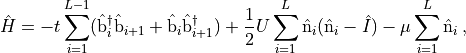
Next we handle the more difficult task of exploring the two parameter phase
space of the Bose-Hubbard Hamiltonian. In one spatial dimension the
Bose-Hubbard Hamiltonian takes the form shown in Eq. (4).
The first term, whose magnitude is controlled by  , is known as the
tunneling term of the model, a large promotes particles tunneling
between nearest neighbor sites. The second term, whose magnitude is controlled
by
, is known as the
tunneling term of the model, a large promotes particles tunneling
between nearest neighbor sites. The second term, whose magnitude is controlled
by  , describes repulsive on site interaction, finally the last term
in the sum accounts for the energy associated with the chemical potential of
the system.
, describes repulsive on site interaction, finally the last term
in the sum accounts for the energy associated with the chemical potential of
the system.
(4)
As usual we begin my importing necessary libraries. There are a couple new
libraries in the lines below. From matplotlib we import cm, this
allows us to use color maps in our plots. This of course requires the
installation of matplotlib.
1import MPSPyLib as mps
2import numpy as np
3import matplotlib.pyplot as plt
4from matplotlib import cm
5from time import time
6import sys
Towards the end of the script we define a function for plotting the results
of our simulations, The function is useful because its sets the limits of
plots using the data provided to it, but not that defining it requires
matplotlib to be installed.
120
121def plotIt(jvalues, muvalues, dependentvalues):
122    """
123    Scatter plot for the phase diagram of the Bose Hubbard model.
124
125    **Arguments**
126
127    jvalues : floats
128        x-values of points
129
130    muvalues : floats
131        y-values of points
132
133    dependentvalues : floats
134        value for coloring points
135    """
136    plt.rc('font', family='serif')
137    plt.rc('mathtext', fontset='cm')
138    plt.scatter(jvalues, muvalues, c=dependentvalues, cmap=cm.jet)
139    plt.xlim((np.min(jvalues), np.max(jvalues)))
140    plt.ylim((np.min(muvalues), np.max(muvalues)))
141    plt.xlabel(r"tunneling  " r"$t/U$", fontsize=16)
142    plt.ylabel(r"chemical potential  " r"$\mu/U$", fontsize=16)
143    cbar = plt.colorbar()
144    cbar.set_label(r"Quantum Depletion", fontsize=16)
145    plt.savefig('02_BoseHubbardStatics.pdf', bbox_inches='tight')
146    plt.show()
147
The first time we run the file, we set the post process flag to False
via the command line argument --PostProcess=False which is passed to
the main function:
10def main(PostProcess=False, ShowPlots=True):
Inside the main function, we set an initial time, this is stored in seconds.
26 t0 = time()
We build the appropriate operators and construct the interaction operator
using the built in linear algebra of python. Note that computationally it
is not necessary to compute the term involving  , since in the
canonical ensemble this only introduces an overall shift in the energy of
the system, the
, since in the
canonical ensemble this only introduces an overall shift in the energy of
the system, the  term
is computed by subtracting the ground state energy
term
is computed by subtracting the ground state energy Output['energy']
across simulations with different numbers of particles.
28    # Build operators
29    Operators = mps.BuildBoseOperators(6)
30    Operators['interaction'] = 0.5 * (np.dot(Operators['nbtotal'],
31                                             Operators['nbtotal'])
32                                      - Operators['nbtotal'])
33    # Define Hamiltonian MPO
34    H = mps.MPO(Operators)
35    H.AddMPOTerm('bond', ['bdagger','b'], hparam='t', weight=-1.0)
36    H.AddMPOTerm('site', 'interaction', hparam='U', weight=1.0)
37
38    # ground state observables
39    myObservables = mps.Observables(Operators)
40    # Site terms
41    myObservables.AddObservable('site', 'nbtotal', 'n')
42    # correlation functions
43    myObservables.AddObservable('corr', ['nbtotal', 'nbtotal'], 'nn')
44    myObservables.AddObservable('corr', ['bdagger', 'b'], 'spdm')
We let OSMPS set the maximum bond dimension using default criteria,
see Sec. Variational ground state search or convergence.MPSConvParam for details.
46 myConv = mps.MPSConvParam(max_num_sweeps=7)
We set U=1, and generate lists for parameters we will change across
simulations. The first is the list of values our tunneling parameter will
range over, tlist, we will sample 20 points from the interval
 . The system size is set to
 L=10 and the number
of particles is set to range from 1 to 11, with 11 sampling points.
48    U = 1.0
49    tlist = np.linspace(0, 0.4, 21)
50    parameters = []
51    L = 10
52    Nlist = np.linspace(1, 11, 11)
Using these lists of numbers we generate all of the necessary parameter lists for our simulation.
54    for t in tlist:
55        for N in Nlist:
56            parameters.append({
57                'simtype'                   : 'Finite',
58                # Directories
59                'job_ID'                    : 'Bose_Hubbard_statics',
60                'unique_ID'                 : 't_' + str(t) + 'N_' + str(N),
61                'Write_Directory'           : 'TMP_02/',
62                'Output_Directory'          : 'OUTPUTS_02/',
63                # System size and Hamiltonian parameters
64                'L'                         : L,
65                't'                         : t,
66                'U'                         : U,
67                # Specification of symmetries and good quantum numbers
68                'Abelian_generators'        : ['nbtotal'],
69                # Define Filling
70                'Abelian_quantum_numbers'   : [N],
71                # Convergence parameters
72                'verbose'                   : 1,
73                'logfile'                   : True,
74                'MPSObservables'            : myObservables,
75                'MPSConvergenceParameters'  : myConv
76            })
If PostProcess=False we run the simulations, check the time in seconds,
and subtract our original time to measure the amount of time mps.runMPS
took to run.
81    # Run the simulations and quit if we are not just Post
82    if(not PostProcess):
83        if os.path.isfile('./Execute_MPSMain'):
84            RunDir = './'
85        else:
86            RunDir = None
87        mps.runMPS(MainFiles, RunDir=RunDir)
88        return
After the simulation data is computed, the Outputs are stored in the local
process, and NumPy arrays are initialized to store the pertinent data. Namely,
a for loop construction is used to build the depletion, energies,
tinternal (time), and chempotmu (chemical potential). See below.
 93    Outputs = mps.ReadStaticObservables(parameters)
 94
 95    depletion = np.zeros((Nlist.shape[0], tlist.shape[0]))
 96    energies = np.zeros((Nlist.shape[0], tlist.shape[0]))
 97    tinternal = np.zeros((Nlist.shape[0], tlist.shape[0]))
 98    chempotmu = np.zeros((Nlist.shape[0], tlist.shape[0]))
 99
100    kk = -1
101    for ii in range(tlist.shape[0]):
102        tinternal[:, ii] = tlist[ii]
103
104        for jj in range(Nlist.shape[0]):
105            kk += 1
106
107            spdm = np.linalg.eigh(Outputs[kk]['spdm'])[0]
108            depletion[jj, ii] = 1.0 - np.max(spdm) / np.sum(spdm)
109
110            energies[jj, ii] = Outputs[kk]['energy']
111
112        chempotmu[0, ii] = energies[0, ii]
113        chempotmu[1:, ii] = energies[1:, ii] - energies[:-1, ii]
The plot should then look like
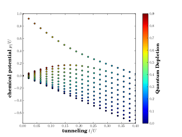
The actual function for the plot looks like
121def plotIt(jvalues, muvalues, dependentvalues):
122    """
123    Scatter plot for the phase diagram of the Bose Hubbard model.
124
125    **Arguments**
126
127    jvalues : floats
128        x-values of points
129
130    muvalues : floats
131        y-values of points
132
133    dependentvalues : floats
134        value for coloring points
135    """
136    plt.rc('font', family='serif')
137    plt.rc('mathtext', fontset='cm')
138    plt.scatter(jvalues, muvalues, c=dependentvalues, cmap=cm.jet)
139    plt.xlim((np.min(jvalues), np.max(jvalues)))
140    plt.ylim((np.min(muvalues), np.max(muvalues)))
141    plt.xlabel(r"tunneling  " r"$t/U$", fontsize=16)
142    plt.ylabel(r"chemical potential  " r"$\mu/U$", fontsize=16)
143    cbar = plt.colorbar()
144    cbar.set_label(r"Quantum Depletion", fontsize=16)
145    plt.savefig('02_BoseHubbardStatics.pdf', bbox_inches='tight')
146    plt.show()
147
148    return
Now we can continue in the next example with a real time evolution.