Example: Static Ising Model
In the following paragraphs we will see how OSMPS integrates with the python
environment in a manner that allows for easy visualization of important
quantities. We will begin by analyzing the file 01_IsingStatics.py given in
the Examples subdirectory of OSMPS. This file performs simulations
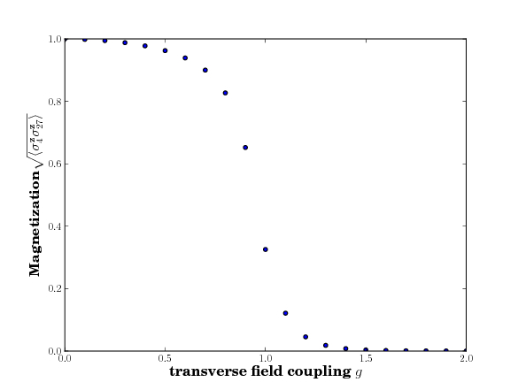
for many values of the transverse field coupling  , and produces a
plot illustrating how the spin correlation between far apart sites changes as
a function of the disorder inducing transverse magnetic field. The
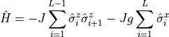
transverse Ising Hamltonian can be written as shown in
Eq. (3), in the file 01_IsingStatics.py we will
understand how to implement in this Hamiltonian in OSMPS, and how we can
study some of its ground state properties.
, and produces a
plot illustrating how the spin correlation between far apart sites changes as
a function of the disorder inducing transverse magnetic field. The
transverse Ising Hamltonian can be written as shown in
Eq. (3), in the file 01_IsingStatics.py we will
understand how to implement in this Hamiltonian in OSMPS, and how we can
study some of its ground state properties.
(3)
The file begins by importing MPSPyLib and NumPy, and it also imports matplotlib.pyplot. This of course requires the installation of matplotlib.
1import MPSPyLib as mps
2import numpy as np
3import matplotlib.pyplot as plt
4import sys
If we call the file from the command line, the main function will be
executed, which takes a logic variable as argument. The default value
PostProcess=False means we have not yet run our simulation. If
PostProcess=True is passed as argument, we have run our simulation
and are now using the file to organize and plot our outputs. When calling
the script from the command line this can be specified via
--PostProcess=F or --PostProcess=T:
7def main(PostProcess=False, ShowPlots=True):
Here we populate Operators with the spin operators defined in the
description of Ops.BuildSpinOperators(). We use these operators to
define the Pauli matrices Operator['sigmaz'] and Operator['sigmax']
using well known operator identities.
23    # Build spin operators for spin-1/2 system
24    Operators = mps.BuildSpinOperators(0.5)
25    Operators['sigmaz'] = 2 * Operators['sz']
26    Operators['sigmax'] = (Operators['splus'] + Operators['sminus'])
Here we construct the Hamiltonian for the transverse Ising model,
the first term couples the z component of spin of nearest neighbor qubits,
the second term couples the qubits to a transverse magnetic field, this
field tends to disorder the qubits with respect to measurement in
the z direction. It is important to note that line 32 implicitly sets
 , this will be done explicitly on line 43.
28    # Define Hamiltonian of transverse Ising model
29    H = mps.MPO(Operators)
30    # Note the J parameter in the transverse Ising Hamiltonian
31    # has been set to 1, we are modelling a ferromagnetic chain.
32    H.AddMPOTerm('bond', ['sigmaz', 'sigmaz'], hparam='J', weight=-1.0)
33    H.AddMPOTerm('site', 'sigmax', hparam='g', weight=-1.0)
Here we specify that we are interested in the correlation of the z-component
of spin among all qubits in the lattice. We associate this observable with
the key 'zz', we will use this key in post processing to obtain the
correlation data OSMPS has computed and stored in output dictionaries.
35    # Observables and convergence parameters
36    myObservables = mps.Observables(Operators)
37    myObservables.AddObservable('corr', ['sigmaz', 'sigmaz'], 'zz')
This line specifies the details of the MPS convergence parameters:
39    myConv = mps.MPSConvParam(max_bond_dimension=20, max_num_sweeps=6,
40                              local_tol=1E-14)
Here we explicitly set , so that as we increase the strength of
the transverse magnetic field coupling , the ground state of the
model will transition from ferromagnetic to paramagnetic. Note that line 44
creates a list of values for the parameter , for each value of
in the list glist another dictionary of parameters is created,
and appended to the list parameters.
42    # Specify constants and parameter lists
43    J = 1.0
44    glist = np.linspace(0, 2, 21)
45    parameters = []
46    L = 30
47
48    for g in glist:
49        parameters.append({
50            'simtype'                   : 'Finite',
51            # Directories
52            'job_ID'                    : 'Ising_Statics',
53            'unique_ID'                 : 'g_' + str(g),
54            'Write_Directory'           : 'TMP_01/',
55            'Output_Directory'          : 'OUTPUTS_01/',
56            # System size and Hamiltonian parameters
57            'L'                         : L,
58            'J'                         : J,
59            'g'                         : g,
60            # ObservablesConvergence parameters
61            'verbose'                   : 1,
62            'MPSObservables'            : myObservables,
63            'MPSConvergenceParameters'  : myConv,
64            'logfile'                   : True
65        })
As mentioned, the simulations will be carried out if PostProcess=False.
72    if(not PostProcess):
73        if os.path.isfile('./Execute_MPSMain'):
74            RunDir = './'
75        else:
76            RunDir = None
77        mps.runMPS(MainFiles, RunDir=RunDir)
78        return
Alternatively, if PostProcess=True then we have already run our simulations
and are only interested in plotting. This brings us to line 72, where, assuming
we have already run our simulations and set PostProcess=True, we pass the
PostProcess if statement. We first initialize the list magnetizationlist
as an empty list. We then use ReadStaticObservables to store the output
dictionaries of our simulations in Outputs. Since each entry in Outputs
is a dictionary, we need to supply the proper key to each dictionary in order to
receive the observable data our simulations have generated. We accomplish this
with lines 80, for each Output dictionary in our list Outputs, we
supply the key 'zz', returned to us is the corresponding observable, in
this case a two dimensional array summarizing the correlations between all
sites in the system. On line 80 we pick out the spin-spin correlation between
sites 4 and 27, these are arbitrary numbers, chosen only to be separated by
many sites, and not directly located at a boundary, and use the square root
of this quantity as an estimate of the magnetization of the system. The
correlation between these two sites is temporarily stored in
spincorrelation, each time we pass through the for loop we append the
new value of spincorrelation to spincorr. Finally lines 61-68 use the
plotting function scatter from matplotlib.pyplot to create a plot of
the magnetization as a function of the disorder inducing transverse magnetic
field, the usetex=True on line 82 allows us to use the built in LaTeX
capabilities in matplotlib.pyplot. Note that any text within quotes
preceded by r, will be parsed as LaTeX. So that if lines 91-102 are to
run without error, you must install matplotlib.
 71    # Run the simulations and quit if we are not just Post
 72    if(not PostProcess):
 73        if os.path.isfile('./Execute_MPSMain'):
 74            RunDir = './'
 75        else:
 76            RunDir = None
 77        mps.runMPS(MainFiles, RunDir=RunDir)
 78        return
 79
 80    # PostProcess
 81    # -----------
 82
 83    magnetizationlist = []
 84    Outputs = mps.ReadStaticObservables(parameters)
 85    for Output in Outputs:
 86        print(Output['converged'])
 87
 88        # Get magnetization from spincorrelation zz
 89        magnetizationlist.append(np.sqrt(Output['zz'][3][26]))
 90
 91    plt.rc('font', family='serif')
 92    plt.rc('mathtext', fontset='cm')
 93    plt.scatter(glist, magnetizationlist)
 94    plt.xlabel(r"transverse field coupling  " r"$g$", fontsize=16)
 95    plt.ylabel(r"Magnetization"
 96               r"$\sqrt{\langle\sigma^\mathbf{z}_4\sigma^\mathbf{z}_{27}\rangle}$",
 97               fontsize=16)
 98    plt.xlim((0, 2))
 99    plt.ylim((0, 1))
100    if(ShowPlots):
101      plt.savefig('01_IsingStatics.pdf', bbox_inches='tight')
102      plt.show()
103
104    return
Running this example we receive the following plot as output.
Alternatively, if you would rather use the plotting capabilities provided by
other programs, the data can easily be written out by substituting the
following code in place of lines 91-99.
The key line in the code below is line 89, this line appends each element of
the Outputs['zz'][3][26] to magnetizationlist where it is used later to
build a scatter plot. A note: [3][26] is a site-pair specification. It
indicates that we are grabbing the two-point correlator for sites 3, and 26
(where the first site is indexed 0).
83    magnetizationlist = []
84    Outputs = mps.ReadStaticObservables(parameters)
85    for Output in Outputs:
86        print(Output['converged'])
87
88        # Get magnetization from spincorrelation zz
89        magnetizationlist.append(np.sqrt(Output['zz'][3][26]))
90
We note that it is a simple matter to add the 'unique_ID' string
to the end of a file name using +, which adds numbers and joins
strings.