Python Module model¶

The models constructed in this module provide a the most simplistic entry to openMPS. For designing more sophisticated Hamiltonians, it is necessary to go through the steps of creating the operators and building an MPO on your own.

Details

Pre-built models return the operators, the MPO, and an observable class. The following pre-built models exist.

Quantum Ising model model.QuantumIsingModel
Bose-Hubbard model model.BoseHubbardModel
Bilinear-Biquadratic spin-one model: BilinearBiquadraticModel

class model._Model[source]¶

Abstract class for any model providing basic functions.

__call__()[source]¶: Use the call attribute to return the classes for operators, MPOs, and measurements.

build()[source]¶: Return the operators, the MPO, and a measurement object.

build_observables()[source]¶: Build an observable class for the bilinear biquadratic model.

class model.QuantumIsingModel[source]¶

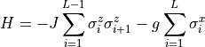
Build the Hamiltonian including the operators and observables class for the quantum Ising model. After creating an instance of the model, you can call the object like a function and it will return a tuple with the operators, the MPO, and the observables class. The Hamiltonian is defined as:

$H = -J \sum_{i=1}^{L-1} \sigma_{i}^{z} \sigma_{i+1}^{z} -g \sum_{i=1}^{L} \sigma_{i}^{x}$

Arguments

No arguments

Details

We choose the Pauli operators to be diagonal in $\sigma^{x}$ which allows to use the $Z_{2}$ symmetry in the Ising model. The following string identifiers are defined for each term in the Hamiltonian:

String identifier	Hamiltonian term
`J`	$\sigma_{i}^{z} \sigma_{i+1}^{z}$
`g`	$\sigma_{i}^{x}$

The following operators are built based on the spin operators:

String	Definition
I	Identity $1$
splus	Spin raising $S^{+}$ (in x-direction)
sminus	Spin lowering $S^{-}$ (in x-direction)
sz	Pauli-z matrix $\sigma^{z}$ (not diagonal)
sx	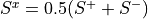$S^{x} = 0.5 (S^{+} + S^{-})$ (diagonal)
gen	Generator for $Z_2$ (0 and 1 on the diagonal)

build_mpo()[source]¶: Build the MPO for the quantum Ising model.

build_operators()[source]¶: Build all necessary operators for the quantum Ising Hamiltonian.

class model.XXXModel[source]¶

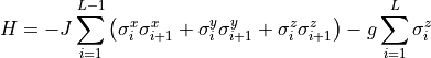
Build the Hamiltonian including the operators and observable class for the spin-1/2 XXX model. After creating an instance of the model, you can call the object like a function and it will return a tuple with the operators, the MPO, and the observables class. The Hamiltonian is defined as:

$H = -J \sum_{i=1}^{L-1} \left( \sigma_{i}^{x} \sigma_{i+1}^{x} + \sigma_{i}^{y} \sigma_{i+1}^{y} + \sigma_{i}^{z} \sigma_{i+1}^{z} \right) - g \sum_{i=1}^{L} \sigma_{i}^{z}$

Arguments

No arguments.

Details

The following string identifiers are defined for each term in the Hamiltonian:

String identifier	Hamiltonian term
`J`	Interaction, i.e., xx-term, yy-term, and zz-term at equal strength.
`g`	$\sigma_{i}^{z}$

The following operators are built based on the spin operators:

String	Definition
I	Identity $1$
splus	Spin raising $S^{+}$ (in x-direction)
sminus	Spin lowering $S^{-}$ (in x-direction)
sz	Spin-z matrix $\sigma^{z}$

build_mpo()[source]¶: Build the MPO for the XXX model.

build_operators()[source]¶: Build all necessary operators for the XXX model.

class model.XXZModel[source]¶

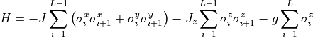
Build the Hamiltonian including the operators and observable class for the spin-1/2 XXZ model. After creating an instance of the model, you can call the object like a function and it will return a tuple with the operators, the MPO, and the observables class. The Hamiltonian is defined as:

$H = -J \sum_{i=1}^{L-1} \left( \sigma_{i}^{x} \sigma_{i+1}^{x} + \sigma_{i}^{y} \sigma_{i+1}^{y} \right) - J_{z} \sum_{i=1}^{L-1} \sigma_{i}^{z} \sigma_{i+1}^{z} - g \sum_{i=1}^{L} \sigma_{i}^{z}$

Arguments

No arguments.

Details

The following string identifiers are defined for each term in the Hamiltonian:

String identifier	Hamiltonian term
`J`	Interaction of xx-term and yy-term at equal strength.
`Jz`	Interaction of zz-term.
`g`	$\sigma_{i}^{z}$

The following operators are built based on the spin operators:

String	Definition
I	Identity $1$
splus	Spin raising $S^{+}$ (in x-direction)
sminus	Spin lowering $S^{-}$ (in x-direction)
sz	Spin-z matrix $\sigma^{z}$

build_mpo()[source]¶: Build the MPO for the XXZ model.

build_operators()[source]¶: Build all necessary operators for the XXZ model.

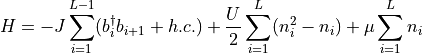
class model.BoseHubbardModel(nmax=4, chem_pot=False)[source]¶

Build the Hamiltonian including the operators and observables class for the Bose-Hubbard model. After creating an instance of the model, you can call the object like a function and it will return a tuple with the operators, the MPO, and the observables class. The Hamiltonian is defined as:

$H = - J \sum_{i=1}^{L-1} (b_{i}^{\dagger} b_{i+1} + h.c.) + \frac{U}{2} \sum_{i=1}^{L} (n_{i}^2 - n_{i}) + \mu \sum_{i=1}^{L} n_{i}$

Arguments

nmaxint, optional: Maximal number of bosons on one site. (If you need spinful or flavorful bosons, minimal number of bosons, etc., you have to go beyond the default models. Default to 4.
chem_potboolean, optional: Specifies if the chemical potential term $\mu$ should be included in the Hamiltonian. Default to False.

Details

The string identifiers for each Hamiltonian parameters are:

String identifier	Hamiltonian term
`J`	math:b_{i}^{dagger} b_{i+1} + h.c. (Tunneling)
`U`	math:n_{i}^2 - n_{i} (On-site interaction)
`mu`	math:n_{i} (chemical potential)

The following operators are built:

String	Definition
I	Identity $1$
bdagger	Creation operator $b^{\dagger}$
b	Annihilation operator $b$
nbtotal	Number operator $n = b^{\dagger} b$
interaction	$0.5 (n^2 - n)$

build_mpo()[source]¶: Build all necessary operators for the Bose-Hubbard model.

build_operators()[source]¶: Build all necessary operators of the Bose-Hubbard Hamiltonian.

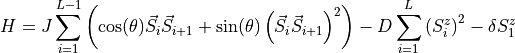
class model.BilinearBiquadraticModel(symmetry_breaking=False, fix_theta=None, use_symm=False)[source]¶

Build the Hamiltonian including the operators and observables class for the bilinear biquadratic model. After creating an instance of the model, you can call the object like a function and it will return a tuple with the operators, the MPO, and the observables class. The Hamiltonian is defined as:

$H = J \sum_{i=1}^{L-1} \left( \cos(\theta) \vec{S}_{i} \vec{S}_{i+1} + \sin(\theta) \left( \vec{S}_{i} \vec{S}_{i+1} \right)^2 \right) - D \sum_{i=1}^{L} \left( S_{i}^{z} \right)^2 - \delta S_{1}^{z}$

Arguments

symmetry_breakingbool, optional: Specifies if a symmetry breaking field should be included in the Hamiltonian. Default to False.
fix_thetafloat or None, optional: If None (default), the more general Hamiltonian with thirteen bond rules is built. If you know that theta is fix for all simulations (statics and dynamics), you may pass the actual value reducing the problem to nine bond rules.
use_symmbool, optional: We can use the symmetry of the Bilinear biquadratic model. This requires that theta is given. A warning is printed that symmetry is not used if theta is not given.

Details

The string identifiers for each Hamiltonian parameter are:

String identifier	Hamiltonian term
`cost`	math:vec{S}_{i} vec{S}_{i+1}
`sint`	math:left( vec{S}_{i} vec{S}_{i+1} right)^2
`D`	math:left( S_{i}^{z} right)^2
`Delta`	math:S_{1}^{z}

The following operators are built.

String	Definition	Comments
I	Identity $1$
splus	Spin raising $S^{+}$
sminus	Spin lowering $S^{-}$
sz	Spin z $S^{z}$
sx	$S^{x} = 0.5 (S^{+} + S^{-})$	Only without symmetry
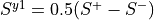
sy1	$S^{y1} = 0.5 (S^{+} - S^{-})$	Only without symmetry
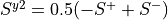
sy2	$S^{y2} = 0.5 (-S^{+} + S^{-})$	Only without symmetry
sx2	$S^{x^2}$	Only without symmetry
sy2	$S^{y^2}$	Only without symmetry
sz2	$S^{z^2}$
sxz	$S^{x} S^{z}$	Only without symmetry
sxy1	$S^{x} S^{y1}$	Only without symmetry
sxy2	$S^{x} S^{y2}$	Only without symmetry
szy1	$S^{z} S^{y1}$	Only without symmetry
szy2	$S^{z} S^{y2}$	Only without symmetry